6 More about instruments
The FM Synth and Sampler are the sound creation powerhouses of the M8. But they each have their limitations. Sound design is not quick or straightforward on the FM Synth. A small change to a parameter can have a large effect, so it can be difficult to modulate over a range of related, pleasing sounds. While it has a large range, having only four operators and limited modulators means that some sounds are just not possible. The Sampler, on the other hand, can play any sound that has been recorded. But one has to find that recording, either by searching on the Internet or through one’s own sprawling and poorly-organized collection. The set of transformations that can be applied to a sample is limited.
Each of these two powerful instruments compensates in part for the deficiencies of the other, but there are still circumstances where the remaining instrument types can be useful, for a particular sound, or for the speed and ease of deploying them. In this chapter, we’ll discuss the remaining sound generation types: Wavsynth, Macrosynth, and Hypersynth. We saw each of these briefly in chapter 3, but we’ll look at them in more detail. We won’t go as deep as we did in chapters 4 and 5, because these instruments are more specialized, and the M8 manual does a good job of covering them. We’ll confine ourselves to overviews and some tips on use.
There are two instrument types that do not directly generate sound on the M8, but are used to control other instruments. The MIDI Out instrument can send sequencing information to another device over a cable, using the global MIDI standard. The External Instrument is a variation on MIDI Out for use when you want to bring the sound made by that other device back into the M8 to send to the effects (chorus/phaser/flanger, delay, reverb) and mix with the sounds on other M8 tracks. MIDI generated by another device or controller (such as a keyboard) can also be used to sequence an M8 track using one of the sound engines above.
Before we get into the details of these instruments, we’ll discuss some general topics that apply to all of them.
6.1 Instrument modulators
In the previous chapters, we mostly used AHD (Attack-Hold-Decay) envelopes, because each of these stages have duration measured in ticks, so we didn’t have to worry about turning notes off in the phrase. We also used some synth models that had an envelope built in (such as the pluck sound in the first song, from Macrosynth) and some samples whose sounds had specific duration (such as the percussion in the first song).
The ADSR (Attack-Decay-Sustain-Release) adds a fourth parameter, sustain, which is not a duration, but a level. The envelope amplitude falls to this level during the decay phase and stays there for the duration of the note. When the note ends, the release phase starts, and the amplitude falls to zero. There is no release phase if the note ends because a new note is triggered, only if the OFF command is used. The diagrams in the M8 manual may be of use in visualizing this. ADSR envelopes were included in Moog synthesizers from the mid ’60’s, and are common on polyphonic keyboard synthesizers. If one plays a piano note and holds the key down, the amplitude is somewhat like ADSR, but it will decay slowly during the sustain phase. Some synthesizers (such as the DX series, but not M8) have additional parameters to implement this.
The drum envelope was added by Tim when he was working on his FM drums pack. It is reminiscent of a diagram in Chowning’s 1973 paper showing how a drum sound can be made from a modulator-carrier pair by adjusting the index (modulator ratio in M8 lingo) with an envelope whose amplitude starts off in the middle, swells, and then decays to zero. Tim has added a sharp attack and partial decay phase with both duration and final level controlled by the Peak parameter; the Body parameter for the swell duration; and the Decay parameter for the duration of the final decay. These durations are measured in milliseconds. The drum envelope thus has aspects of both AHD and ADSR envelopes, and its primary use is on the ratio of FM modulator operators. But, of course, it can be used to modulate all the other destinations as well, and on instruments other than FM Synth.
The trig envelope is like AHD, but it is bipolar, and one chooses an instrument or track as the trigger source (usually a different one, but that’s not necessary). The primary use case is for "ducking". This is an effect often caused by the use of a compressor, which limits the dynamic range of sounds. When there is a sharp increase in volume, such as caused by a kick drum hit, it can cause the compressor to turn down the volume, which sounds like all the already-playing instruments "ducking" to let the kick drum sound. This is highly prized as a dancefloor rhythm. M8 does not have a compressor (though it is frequently wished for), but one can simulate the effect to some extent using trig envelopes with negative amount to turn down the volume of other sound sources on kick hits. Again, since it is a general effect, you can think of other uses.
More complex envelopes can be created using tables, as we’ll explain in a later chapter. The same is true for LFOs.
Each envelope shape is a different instrument modulator type. In contrast, there is only one LFO type, but several different shapes and behaviours can be configured within it. Once again, there are diagrams in the M8 manual to help you. We’ve mostly been using the triangle shape, which is a smooth back-and-forth with abrupt changes at the extremes. The sine shape slows to a halt at the extremes, which can make a subtle difference in some circumstances. There are other shapes familiar to us from audio-rate oscillators: ramp up and down (like a saw wave), and square up and down (differing on whether it starts at zero or finishes there). Then there are exponential down and up shapes, and finally two random shapes. "Random" is stepped; a pseudo-random source is sampled and held for the duration of the cycle. But "Drunk" is continuous, like an inebriated person trying to walk home.
There are four LFO behaviours, two looping and two "one-shot" (that is, the shape is only traversed once). The two looping behaviours differ in whether or not the LFO resets to the start of its shape on each trig. In Free mode, it does not; in Retrig mode, it does. The two one-shot behaviours differ on what value is held after the shape is traversed. In Once mode, the final held value is the start value; in Hold mode, it is the last value of the shape.
LFOs are unipolar except when applied to two specific destinations, Pitch and Pan. We described ten shapes above, but there are actually twenty choices for the shape setting, because the first ten have periods measured in steps, but they repeat with the second ten having periods measured in ticks. A "T" is added to the end of the shape to remind you of this.
The final instrument modulation type is Tracking. This lets one create a numerical value from note frequency or velocity that can be applied to the standard set of destinations. There are actually three choices, the third one disconnecting the velocity from affecting volume like it usually does. These choices are made with the Src (source) setting. Two additional parameters, lval and hval, specify the points in the source to map to zero and max amount respectively. That is, you can have the tracking apply to only a subrange of the source, and if lval is greater than hval, the modulator will decrease as the source increases.
The most common destinations for this modulation is probably filter cutoff. If you are applying, say, a lowpass filter with some resonance, and not using tracking, then as you play higher notes, the resonance will no longer have as much effect, and the volume will start to drop off. What you really want is for the filter cutoff to track note frequency, so that the effect on the higher notes remains the same. User impbox on the Discord has figured out the magic values to keep note and filter aligned: cutoff 20, tracking amount 82, lval 00, hval 54. You might have to do some experimentation to find similar values if you are putting this feature to another purpose.
Another useful destination is modulator amount on the FM Synth. Higher notes don’t need as many even higher harmonics added to them, and to properly simulate some real-world instruments, the FM modulation needs to be reduced. This can be done with a tracking modulator whose source is frequency (an example of where you want lval to be greater than hval). Using this kind of modulator with velocity as the source and filter cutoff as destination can give a similar sort of damping effect where notes of higher frequencies are less complex (a piano works this way, for example).
One modulation destination that is worth highlighting is another modulator, known colloquially as a "mod mod". A common use is to apply an LFO to the frequency of another LFO to turn it into an even more complex modulation. There wasn’t really space in the user interface to allow specifying any other modulator as the destination, so if this type of destination is chosen on modulator 1, then it can only affect modulator 2. Similarly, modulator 2 can only affect modulator 3, and so on in a circle, so modulator 4 can only affect modulator 1. If the destination is Mod Amt, then the amount of the destination modulator is reduced by a multiplicative factor specified by the mod mod. The destination Mod Rate will affect all time parameters on the destination modulator, again in a multiplicative fashion. Finally, there is Mod Both. If you only want to affect one parameter, such as decay but not attack, you will need to use FX commands in a phrase or table.
While we are talking about things visible in Instrument View, it may be a good time to note that navigating up a screen gets us to Instrument Pool View, introduced in firmware 4.0.0. It is visible in the mini-map as a P above the M representing Instrument Modulation View. Here is the Instrument Pool View for the demo song for M:02.
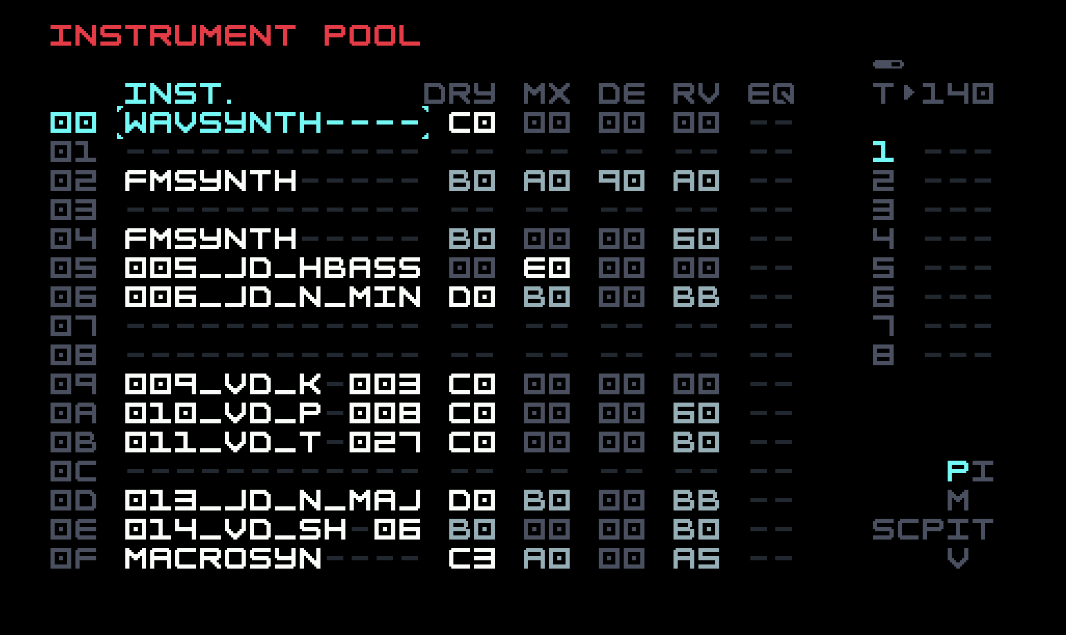
You can see that an I has appeared in the mini-map to the left of the highlit P representing the current position, meaning you can quickly get to Instrument View for an instrument listed just by putting the cursor on it and navigating right. Navigating left from there will return you to Instrument Pool View. The view also lets one control all dry volumes, as well as modfx, delay, and reverb sends, and change or quickly access the assigned EQs for each instrument.
There are button combos to reorder instruments in the table, and M8 takes care of renumbering all instrument references elsewhere, if you change the number of an instrument this way. There are also two other ways to get to Instrument Pool View. For details, and more useful shortcuts, we refer you to the M8 manual.
6.2 Scales and transposition
We have already seen a few places where transposition (moving all notes by a set amount) is made easy on M8. We used it for an easy variation in our first song, because there is a transposition column in Phrase View, and we’ve also seen that there is a similar column in tables, though we haven’t used it yet (see chapter 7).
If you don’t know any music theory, this is not the place to learn it, and if you do, you will likely find something annoying (hopefully not everything) in the brief overview that follows. But we’ll persevere.
We described in chapter 3 the mini-keyboard display visible in several views in terms of a single octave on a piano keyboard, the lower row being the white keys (with names like C, D, E, F, G, A, B) and the upper row being the black keys (names modified like C-# or C-sharp on the M8, but also called D♭ or D-flat). We also alluded to our songs in chapters 3 and 4 being in the scale of C minor, because of a few sharps/flats we used.
If we stick to the white keys, and furthermore make C our root note, the place from which we depart and return to, then we are using the scale of C major. But if we do the same thing, but make A the root note, we are using the scale of A minor. The difference can be heard by playing the seven note sequence C, D, E, F, E, D, C (in C major), and then the seven note sequence A, B, C, D, C, B, A (in A minor). Major scales sound more cheery and sunny; minor scales more dark and gloomy. Of course, this is not a firm distinction; one can write a lovely uplifting melody in a minor key, or something miserable in a major key. The difference between major and minor scales is in the placement of the one-semitone jumps as opposed to the two-semitone jumps. (This discussion is complicated by multiple variations on minor scales, at least one of which varies going up versus going down, but never mind about that now.) To get to the C minor scale we used earlier, we just move the root from A to C; that is, we transpose every note up three semitones.
If we take a melody written in C major (using only white keys) and transpose it up one semitone, we potentially use all five black keys and two white keys within an octave. (This is the key of C# major.) When we used transpositions for variations in chapter 3, we were careful in our choice of how much, so we only needed to transpose the pluck and bass, and nothing else. If we had transposed our two tracks up one semitone, it would have sounded bad, unless we transposed everything, in which case it would just sound a bit odd, and only in the transition. Some other transpositions (of only some tracks) sound reasonable and yet others sound bad again. We could smooth things out a bit if we insist that a transposition respect the scale; in our example, that we move any notes that land on black keys to the nearest white key (with some systematic way of choosing when there are two options). In a nutshell, this is a feature that M8’s extensive scale settings provide.
But first, transpositions. In addition to the transposition columns we have seen in chains and tables, there is a global transpose in Project View, with an option in Track View to exclude a particular track from this. Global transpose is intended for use in performance. We have also seen a very local transposition with the PIT command, which we used to build the chord stab in chapter 4. All of these (and others to be described later) will respect the scale options we will now describe.
When in Groove View (which, remember, is above Phrase View), the mini-map shows an S above the G, which is Scale View. Navigating up gets us to Scale View.
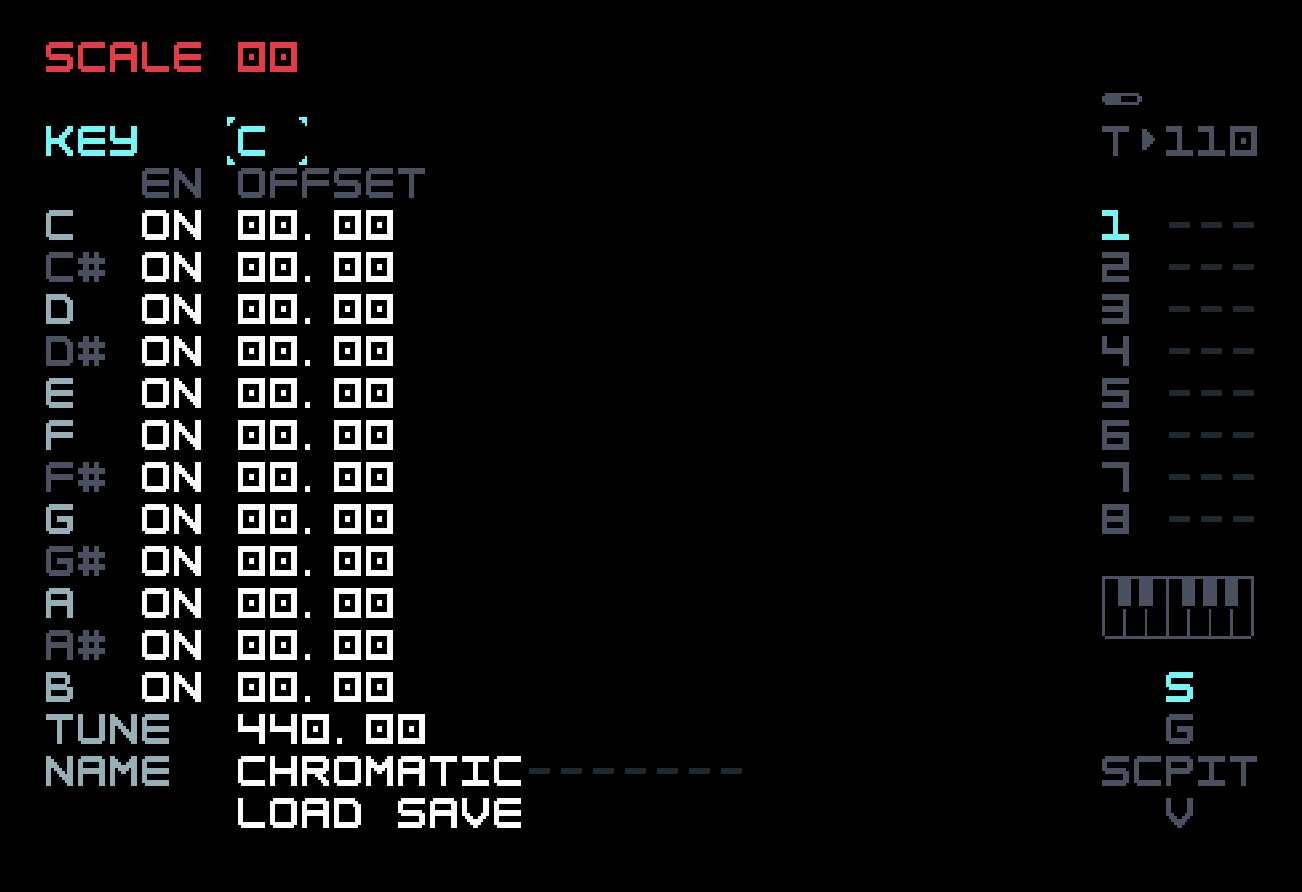
This looks complicated, but the important thing to notice is at the bottom, where there is a name field and options to load and save. While you can make your own scales (and we’ll explain how), there are 92 factory scales provided, including variations on major, minor, and pentatonic (based on the five black keys in an octave), and the seven Greek modes. These provided scales aren’t built in, any more than the factory instruments; they can be deleted, modified, or tweaked and variations saved.
Sixteen different scales can be available in a project. The default scale (global across the project) is scale 00, and in a new project this defaults to C chromatic, that is, all twelve familiar semitones are available. This is the scale we’ve been using this far. There is a row in Project View where the global scale can be set, and Scale View for that scale can be reached from there also.
The top row, labelled "Key", specifies the root note of the scale. Changing it also changes the top row of the 12-semitone table that follows. That table has note labels in the first column, and an enable/disable switch for each note in the second column. To build a C major scale (instead of just loading it from the factory scales), we could switch off all the sharp (#) notes. The last column is an offset in semitones, with separately-editable fields before and after the decimal point (as we had with FM ratios). By setting the offset in the C row to 02.00, we could make a C entry in a phrase play as D, if we wanted to. It’s probably more useful to edit the field after the decimal point, if you want to do microtonal work. At the bottom, just above the name field, is an option to change the global tuning, with the value of A-6 given in Hertz (default 440).
We wrote our previous songs in the key of C minor, even though we didn’t specify this (we were using the default C chromatic scale). We just avoided using the notes that weren’t in C minor, and you can do the same. The value of using an M8 scale is more evident when doing transpositions or altering pitch with randomization. While sticking to a major or minor scale will not guarantee consonance, it makes more pleasant sounds more likely. You could guarantee consonance by building a "scale" that only has notes of a pleasant chord, or even just one note (quantization to octaves). Scales can be set on a per-track basis by using the FX command SCA. The value provided will specify both the scale and the key. The SCG command will set the global scale.
6.3 Wavsynth
Although the amplitude resolution of M8 is 16 bits (so 2 to the power of 16 or 65536 different values are possible), Wavsynth is an 8-bit synthesizer, meaning it deliberately only uses 2 to the power of 8 or 256 different values. You can see the effect of this using the oscilloscope, if you listen to a waveform like saw. It looks like a staircase rather than a ramp. Those vertical edges add more higher harmonics to the sound, making it seem brighter, as if coming out of a small, inexpensive speaker. These higher harmonics can be filtered away, but you will not reclaim clean waveforms, for the most part.
We deliberately chose Wavsynth for our first melodic sound in our first song in chapter 3, though we carefully chose a waveform which looks the same in either resolution. It’s true that Wavsynth is primarily intended for chiptune. However, it’s entirely possible that you could find a use for it in other contexts, especially in a mix with other instruments.
Wavsynth is simple enough that you can explore it on your own, with the help of the M8 manual. One thing you may find puzzling is the inclusion of three extra filter options. These are essentially 8-bit filters, as they alter the waveform in an approximation of what a filter would do, while conforming to the 8-bit restriction. Consider them as just another way to alter the sound.
Added in firmware 4.0.0 are a number of shapes which are wavetables. A wavetable is a series of related waveforms, like frames of a movie. The idea is to modulate the sound by changing position in the table. The Scan parameter is the way to do this. Earlier firmware only offered the Overflow shape which just used the contents of whatever was next in the firmware (with mostly noisy effects). If the filter is off or set to one of the WAV filters, the oscilloscope is also off, and shows the static waveform. This is useful for on-the-fly selection without having to look at the graphic depictions in the manual.
6.4 Macrosynth
We’ve already mentioned that Macrosynth uses code from the Eurorack module Braids by Mutable Instruments. This is a good choice for a number of reasons, not only because it is a reuse of open-source code that was very popular in another synth community, but because a Eurorack module also has to cope with user interface limitations due to size, and code for digital Eurorack modules also has to respect the modest processing chips used in their builds.
The original Braids module was close to the size of the M8 (13 x 8cm), with a 4-digit seven-segment display, one push encoder for editing, six knobs for control, five input jacks and one output jack. We’ve already seen the "macro" approach, where one parameter controls several others, used with the op-mods in FM Synth, but there we had some control over configuration. With Braids and Macrosynth, for better or for worse, we have only two major controls (Timbre and Color) and no say in how they affect each model.
This also leads to a certain vagueness in the documentation, because we don’t know what those hidden model parameters being controlled are or what they do, and part of the point is to not worry about things like that. Neither the official Mutable Instruments documentation nor the unofficial illustrated guides and cheat sheets created by the Eurorack community are much more illuminating than the M8 manual, which has a main section on Macrosynth plus a description of each model in an appendix. The bottom line is that you have to try each one and see what it can do for you.
The 48 models (chosen by the Shape parameter) can be divided into a number of categories: virtual analog (VA), digital, vocal, additive, FM, physical modelling, percussive, wavetables, noise.
"Virtual analog" is a term used to refer to software emulations of classic analog synthesizers, usually using subtractive synthesis, where a restricted class of waveforms is available for later processing with voltage-controlled amplifiers and filters. It’s worth noting that the VA options here cover most of what Wavsynth can do, but in full 16-bit fidelity (and what isn’t covered here is covered further down). The VA model range from 00CSaw to OF Saw Comb.
The "Digital" models aren’t trying to simulate analog, but rather simulate classic digital, somewhat reminiscent of Wavsynth. The models here include 10 Toy and 11 - 14 Digital Filters, which resemble the emulated filters of Wavsynth, but again in full fidelity.
The "Vocal" models use a technique called formant synthesis, based on the idea that three bandpass filters tuned to specific frequencies can sound like elongated vowels. This is not lifelike speech, but something vaguely reminiscent of warmup exercises a choir might do. The models are 15 Vosim through 17 Vowel FOF.
There is one "Additive" model, 18 Harmonics. Subtractive synthesis takes a harmonic-rich waveform like saw and subtracts harmonics using filters. Additive synthesis adds harmonics to the fundamental sine wave, a technique that is expensive in the analog realm but feasible digitally. With only two parameters to control the added harmonics, the possibilities are limited, but it’s worth noting that, in contrast to FM Synth offering a fixed choice of operator waveforms, the Elektron Digitone has a parameter that morphs through additive waveforms in a manner similar to this model.
There are three models that use two-operator FM, from 19 FM to 1B Chaotic Feedback FM, and you may enjoy contrasting these with FM Synth.
Physical modelling is probably the most compelling of the categories offered by Macrosynth, though one has to keep in mind that the computational resources are limited, so one will not get startling fidelity, but rather something that gets reasonably close to the real thing. We’ve already put 1C Plucked to good effect in the lead of our first song in chapter 3. The other models are 1D Bowed, 1E Blown, 1F Fluted, 20 Struck Bell, and 21 Struck Drum. You may enjoy comparing these last two to FM Synth, but there are no equivalents for the others.
There are three models in the "Percussive" category, and they are not included in the previous paragraph because they do not emulate physical instruments but electronic ones, in this case the Roland TR-808. The models are 22 Kick, 23 Cymbal, and 24 Snare, and you might enjoy comparing these to the samples from the original included in the M8 factory content. These can be tweaked in ways that a sample cannot (hence the number of samples included in the content), so they may be more amenable to modulation or automation.
The next category is "Wavetables", and at least some of these have been ported to the 8-bit Wavsynth by Tim, based on the brief labels seen on the M8’s screen. They range from 25 Wavetables to 28 Wav Paraphonic. This last model is one of the few places where chords can be built on M8 in a single track (the others are the multi-carrier FM Synth models, used for example in the dub stab in chapter 4, and Hypersynth below).
Finally, Macrosynth offers several types of noise, from 29 Filtered Noise through to 2F Morse Noise. Putting these through a resonant filter, distortion via a limiter option, and send effects can be rewarding, especially with lots of modulation.
That’s a lot to explore, so take your time doing so.
6.5 Hypersynth
Hypersynth was the last synthesis engine to be added to M8. This was possible mostly because the saw waveform is very simple to compute, and algorithms managing collections of closely-related saws have been developed. The range of sounds that Hypersynth can make is limited, but they are very compelling sounds. You’ve already heard it in the pad in the first song in chapter 3.
Hypersynth offers twelve saw voices, in six pairs. Each pair can be tuned to a separate note, as we’ll explain. The two voices in each pair can be simultaneously detuned using the Swarm parameter, and the voices can be spread in the stereo field using the Width parameter. This sounds quite nice. At some point, the detuning becomes dissonant, but if you keep increasing it, it approaches a consonant interval again. There is a sub-oscillator available, either two octaves below the root note (the one specified in the phrase) or one octave below, and the choice and amount is controlled by the Subosc parameter.
Each of the pairs can be tuned to a different note using the six fields in the Chord row. Hypersynth is scale-aware, that is, one can specify a scale from the project pool, or use the global scale. The note choices are relative to the scale. For example, if the scale is the default C chromatic and a C-4 note is used in the phrase, then to play an E-4, one would use 04 (four semitones) in a chord field. But if the scale is C major, to play an E-4, one would use 02 (two notes up, C - D - E).
Six notes in a chord is a lot, and you might not want to use them all at once. The Shift parameter provides an alternate approach, cross-fading between the first three pairs and the second three. So one could put a different triad (three-note chord) on each, and then switch from one to the other, or smoothly cross-fade (if the chords permit this mixing). You can also clear any voice (using [EDIT]+[OPTION]) and it will not sound.
Each instrument of Hypersynth type can store sixteen chords, and there is an FX command (CRD) to choose among them in a phrase or table. It’s a bit of work to set up the chords, but copy/paste works well on them, and you can look for community instruments already set up, though since one can’t name chords, you will have to decipher them from the numerical information shown, unless the source has additional documentation.
Although we have now described all the opportunities for polyphony within an M8 instrument, it is still possible to coordinate multiple instruments, as we’ll describe in chapter 9.