4 PRIMP: A primitive imperative language
\(\newcommand{\la}{\lambda} \newcommand{\Ga}{\Gamma} \newcommand{\ra}{\rightarrow} \newcommand{\Ra}{\Rightarrow} \newcommand{\La}{\Leftarrow} \newcommand{\tl}{\triangleleft} \newcommand{\ir}[3]{\displaystyle\frac{#2}{#3}~{\textstyle #1}}\)
This chapter continues the development begun in the previous one, by describing the PRIMP machine language, designing a simulator for it, describing the A-PRIMP assembly language, designing an assembler from A-PRIMP to PRIMP, and designing a compiler from SIMP to A-PRIMP, before concluding with a number of variations of SIMP that add additional language features, and discussing how the compiler might handle them.
4.1 A primitive imperative language
Our SIMP simulator uses many high-level features of Racket, notably the ability to manipulate S-expressions. What if we want to move it closer to a more realistic view of memory? It turns out that this suggests simplifications to the language, and I’ll call the result PRIMP, for "primitive imperative language". PRIMP will be an intermediate step, just for pedagogical purposes; the next language, FIST, will be a reasonably faithful version of an actual machine language.
Modern computers put both programs and data into memory. To approach this situation, we will use one vector as our main data structure, to hold both the program and its data. I’ll call this vector "PRIMP memory" (or just "memory" at times). Because the program will be able to change the data in PRIMP memory through mutation, it can also potentially change itself. This is actually on occasion useful in practice, particularly in embedded systems where memory is very constrained. However, programs that do this kind of self-modification are very susceptible to bugs that are hard to track down (as you can easily imagine), and I will avoid this technique here.
We have already seen that the main advantage of vectors is constant-time access to any element. The disadvantage of vectors is that they have a fixed size, and lack the flexibility of lists. In particular, when executing a sequence of statements, we used rest to simply remove the first statement, exposing the next statement to be executed. This technique will not work with a vector.
Consequently, I will change the way we deal with the program; it will remain fixed and unchanged throughout the computation. One PRIMP statement will be stored in one element of PRIMP memory. We will instead keep track of where we are in the program, using an index into PRIMP memory. This index is typically called the program counter (abbreviated PC). It will be a Racket variable holding the index or location of the next statement or instruction to be executed.
Our simulator, like real computers, uses a a fetch-execute cycle. It repeats the following actions: Fetch the instruction at the location indexed by the PC, increment the PC (so that the next instruction is the next one to be fetched), execute the fetched statement.
We could put the program counter into a PRIMP memory location, but for clarity, we will put it into a separate variable in our simulator. As we will see, in the FIST architecture, and in real processors, it is not stored in memory, but in a separate location.
PRIMP will no longer have named variables. Each integer variable will be stored in one element of PRIMP memory. We will use memory locations that come right after the ones used to store the program.
In a real processor, each memory location holds a fixed number of bits (32 or 64), and each primitive operation takes constant time to execute. We will achieve this goal with FIST, the next language. With PRIMP, we will try to make progress towards this goal. We will not limit the range of an integer variable; as with SIMP, its value can be unbounded.
However, a SIMP statement can contain an arbitrarily complex arithmetic or Boolean expression, and we will not permit this with PRIMP. We solve the space problem for expressions by expanding them into a sequence of statements, each of which takes up constant space.
One arithmetic statement will have three arguments: two operands and one destination. Each of these can be a vector index (PRIMP memory location). But we also want to allow numeric operands. We adopt the convention that using 2 as an operand refers to the number 2 (this is called an immediate operand), but using (2) as an operand refers to the PRIMP memory location of index 2 (this is called an indirect operand). Here is an example of an arithmetic statement.
(add (5) (1) (2))
The effect of executing this statement is that the values stored in PRIMP memory locations 1 and 2 are added together, and the result stored in PRIMP memory location 5. We can describe this effect in concise notation that happens to refer to memory in a fashion very similar to that of array references in C and other imperative languages, as well as describing mutation in a manner similar to the way we mutated state variables in our description of mutable ADTs.
\(M[5]\leftarrow M[1]+M[2]\)
I will not define this notation precisely, nor will I give a grammar and semantics for PRIMP and the following language, FIST. It is not difficult to use the techniques we have discussed in earlier chapters to do this. But because we are not proving things about programs in these languages (though it is possible), and because we are writing simulators in Racket, here I will stick to illustrative examples.
The following statement increments an integer variable stored at PRIMP memory location 7. This is a common operation inside SIMP loops.
(add (7) (7) 1)
In these operations, the operands can be immediate values, but the destination must be a memory location (indirect).
Here is the full set of arithmetic operations:
add sub mul div mod
We can treat comparisons and logical operations in the same way. The comparison operations are:
| equal not-equal |
| gt ge lt le |
The logical operations are:
land lor lnot
We are permitting memory locations to contain Boolean values as well as integer values. To use an "immediate" Boolean value, we can use #t and #f. It could happen that, at run time, a logical operation is applied to an integer value, which should result in an error. We can either rely on Racket’s run-time type checking to catch this error, or catch it ourselves in the simulator. Once again, we are in a transitional situation. The structure of SIMP programs precluded this kind of error. Looking ahead to FIST programs, there will be no notion of types associated with values; every value is a 32-bit quantity, which can be interpreted as we see fit.
We can move information from one memory location to another with move. The following expression:
(move (10) (12))
has the following effect:
\(M[10]\leftarrow M[12]\)
The shift from lists to a vector as the primary data structure complicates how we handle conditional execution and repetition. It’s not obvious how to quickly locate the next statement to be executed in an iif or while (if the body contains several statements). Consequently, we replace these two high-level constructs with two simpler statements: an unconditional jump, and a conditional branch.
(jump 12)
Effect:
\(PC\leftarrow 12\)
(branch (20) 12)
Effect:
If \(M[20]\) then \(PC\leftarrow 12\)
Finally, we have two flavours of print, for PRIMP values (immediate constants or contents of memory locations), and for strings.
| (print-val 21) |
| (print-val (15)) |
| (print-string "\n") |
| add sub mul div mod |
| equal not-equal gt ge lt le |
| land lor lnot |
| jump branch |
| move |
| print-val print-string |
A program is a sequence of instructions and Racket values. It is loaded into the memory vector, one instruction per vector element. Execution starts with the instruction at index zero. The program halts on the first attempt to fetch and execute a non-instruction (an integer or Boolean value, as all instructions are lists).
Here is an example SIMP program from the previous chapter:
| (vars [(x 10) (y 1)] |
| (while (> x 0) |
| (set y (* 2 y)) |
| (set x (- x 1)) |
| (print y) |
| (print "\n"))) |
And here is one possible translation into PRIMP. I have made particular choices in translation which are not necessarily the best or most optimal in any sense.
| (gt (11) (9) 0) ; 0: tmp1 <- x > 0 |
| (branch (11) 3) ; 1: if tmp1 goto 3 |
| (jump 8) ; 2: goto 8 |
| (mul (10) 2 (10)) ; 3: y <- 2 * y |
| (sub (9) (9) 1) ; 4: x <- x - 1 |
| (print-val (10)) ; 5: print y |
| (print-string "\n") ; 6: print "\n" |
| (jump 0) ; 7: goto 0 |
| 0 ; 8: 0 [number, halts program] |
| 10 ; 9: x |
| 1 ; 10: y |
| 0 ; 11: tmp1 |
We need a way of actually running this program, namely a PRIMP simulator. This is relatively easy to code in Racket with the imperative features we have learned.
4.2 The PRIMP simulator
We start with the state variables, which in this simple version are global. A more sophisticated version of the simulator would encapsulate them so as to allow for the possibility of running several different machines.
| (define mem (make-vector MEM-SIZE 0)) |
| (define pc 0) |
| (define halted? #f) |
In this summary, I’ll omit most safety checks present in the complete code (which is linked in the Handouts chapter). A good example of where safety checks can be inserted is to catch attempts to access the memory vector using an out-of-bounds index. Of course, Racket will catch this at run time, but it would be more helpful to the user to provide a specific error message, perhaps with additional information.
| (define (mem-get i) |
| (vector-ref mem i)) |
| (define (mem-set! i newv) |
| (vector-set! mem i newv)) |
The function load-primp consumes a list of PRIMP instructions, initializes memory and the halted? flag, and loads the instructions starting at location zero.
| (define (load-primp prog-list) |
| (set! halted #f) |
| (vector-fill! mem 0) |
| (for [(i MEM-SIZE) |
| (c (in-list prog-list))] |
| (mem-set! i c))) |
The function run-primp implements the fetch-execute cycle by simply repeating one fetch-execute step. Note that the PC is incremented after the instruction is fetched, but before it is executed. This is common in processors, for practical reasons. The execution of one instruction is carried out by a "dispatch" function. If a non-list value is encountered as the result of fetching an instruction, the simulated machine stops.
| (define (run-primp) |
| (let loop () |
| (unless halted? |
| (fetch-execute-once) |
| (loop)))) |
| (define (fetch-execute-once) |
| (define inst (mem-get pc)) |
| (cond |
| [(list? inst) |
| (set! pc (add1 pc)) |
| (dispatch-inst inst)] |
| [else |
| (set! halted? #t)])) |
Each instruction is implemented by a Racket function consuming the arguments of the instruction. Here I’ll present only a representative fraction of the implementation functions, and not all of them.
| (define (print-string s) |
| (printf "~a" s)) |
| (define (print-val op) |
| (define val (get-op-imm-or-mem op)) |
| (printf "~a" val)) |
The situation where we have to decode an operand that might be an immediate value such as 7 or a memory reference such as (10) is handled by the function get-op-imm-or-mem.
| (define (get-op-imm-or-mem op) |
| (match op |
| [(? number? v) v] |
| [`(,i) (mem-get i)] |
| [x (primp-error "Bad operand: ~a\n" op)])) |
There are similar functions get-op-mem and set-dest!.
The arithmetic functions are handled by one common curried function bin-num-op. Note the Racket syntax for writing a curried function: bin-num-op consumes one argument (the actual arithmetic function to be applied such as +) and produces a function that consumes the two operands and makes the required change to PRIMP memory. Logical operations are handled similarly.
| (define ((bin-num-op op) dest src1 src2) |
| (define opnd1 (get-op-imm-or-mem src1)) |
| (define opnd2 (get-op-imm-or-mem src2)) |
| (set-dest! dest (op opnd1 opnd2))) |
| (define add (bin-num-op +)) |
| (define (move dest src) |
| (set-dest! dest (get-op-imm-or-mem src))) |
| (define (jump val) |
| (set! pc val)) |
| (define (branch opnd loc) |
| (define tested (get-op-mem opnd)) |
| (when tested (set! pc loc))) |
We map instruction names to the functions
that execute them with a dispatch table
(in this case an immutable hash table, as discussed in the previous chapter).
| (define dispatch-table |
| (hash |
| 'print-val print-val |
| 'print-string print-string |
| 'add add |
| 'sub sub |
| ...)) |
| (define (dispatch-inst inst) |
| (apply (hash-ref dispatch-table (first inst)) |
| (rest inst))) |
That concludes the basic design of the PRIMP simulator. To test it, we can use the PRIMP program I wrote above. The full program is linked in the Handouts chapter.
From looking at the sample PRIMP program, it should be clear that writing a PRIMP program can be quite awkward and time-consuming. Not only are there many small steps to think of and code, but if we were to modify a program, it would likely change the number of statements, which changes the location of the numerical data. We then have to edit all references to that data.
There are at least two ways that we could make this process easier. One is to write a compiler that consumes a SIMP program and produces a PRIMP program. The other is to write an assembler that provides a few useful features for writing PRIMP. Examples of useful features include variable-like names for memory locations and constants, and labels for the target of jump-imm and branch operations.
We will pursue both of these options, first the assembler and then the compiler, and then look into adding more features to SIMP.
4.3 The PRIMP assembler
It makes sense to write the assembler first. Then the compiler can produce a program written in the assembly language which is what the assembler handles. I’ll call this language A-PRIMP.
A-PRIMP adds some pseudo-instructions to PRIMP. The most easily explained looks like this:
(lit 4)
Here "lit" stands for "literal". This is just a way of specifying that the sequence of instructions contains the Racket value 4 at this point. It is only a cosmetic improvement for readability. For a similar reason, the pseudoinstruction (halt) just produces a 0 in the sequence of instructions, since any non-list value will terminate execution if it is fetched.
The next feature is more useful.
(const NAME 6)
This declares the symbol NAME to have value 6. Here we are not using "symbol" in the Racket sense, but in the more general sense of "symbolize". This use of the word is common in this context even when Racket (or Scheme) is not involved. The effect of this pseudo-instruction, which does not result in an actual entry in the sequence of PRIMP instructions, is to be able to use NAME anywhere in the A-PRIMP program that the immediate operand 6 might appear. Here we are following the common convention that symbols in assembler are written in upper case, though this is not necessary (and by no means universal).
The following pseudo-instruction also creates a similar symbol-value binding.
(label NAME)
Once again, no actual entry in the sequence of PRIMP instructions is produced, but NAME is bound to the index of the memory vector where the next actual instruction would be loaded. In other words, we can now use NAME in the program as the target of jump or branch instructions.
We can combine the ideas of label and lit with the data pseudo-instruction.
(data NAME 1 2 3 4)
Here NAME has the value of the index of the memory vector location where the first data item (the 1) is stored, and can be used in place of any indirect operand. The following data items (2, 3, and 4) are stored in consecutive memory locations following the first one. There is a further abbreviation possible:
(data NAME (10 1))
This is equivalent to (data NAME 1 1 1 1 1 1 1 1 1 1) (in which the 1 occurs ten times).
The symbol NAME can now be used where an indirect operand would be written. The translation of (add NAME NAME 1), assuming the data is stored at memory location 40, would be (add (40) (40) 1).
A symbolic name defined in a data statement can also be used as an immediate operand in a data statement. The translation of
| (data X 1) ; assume stored at location 50 |
| (data Y X) ; assume stored at location 51 |
would be
| 1 |
| 50 |
Here is the previous program rewritten to take advantage of these features.
| (label LOOP-TOP) ; loop-top: |
| (gt TMP1 X 0) ; tmp1 <- (x > 0) |
| (branch TMP1 LOOP-CONT) ; if tmp1 goto loop-cont |
| (jump LOOP-DONE) ; goto loop-done |
| (label LOOP-CONT) ; loop-cont: |
| (mul Y 2 Y) ; y <- 2 * y |
| (sub X X 1) ; x <- x - 1 |
| (print-mem Y) ; print y |
| (print-imm "\n") ; print "\n" |
| (jump LOOP-TOP) ; goto loop-top |
| (label LOOP-DONE) ; loop-done: |
| (halt) ; halt |
| (data X 10) |
| (data Y 1) |
| (data TMP1 0) |
The assembler operates in two phases. In the first phase, a hash table is set up with symbols as keys. The associated values may be other symbols whose values are not immediately evident, as the example below shows.
| (const A B) |
| (const B 10) |
In the second phase, the assembler resolves the mapping so that it is represents a mapping from symbol to numeric value (possibly with additional information associated). One possible error to watch for is a series of references that are circular.
| (const A B) |
| (const C A) |
| (const B C) |
Once this resolution is done, a second pass over the program produces the corresponding PRIMP program.
Exercise 12: Complete the implementation of the A-PRIMP to PRIMP assembler. \(\blacksquare\)
4.4 The SIMP to A-PRIMP compiler
Consider the translation of a small program.
| (vars [(x 3)] |
| (print x)) |
SIMP variables become A-PRIMP data statements (after the code for the body of the vars statement). We need to be careful to not have the names in the data statements for variables collide with names we create for other purposes. One way of ensuring this is to prefix the name of each SIMP variable with an underscore character "_", and make sure that none of the other names we generate start with an underscore. This is a standard convention in compilers.
The function compile-statement produces a complete program when given a vars statement. For other statements, compile-statement produces a partial program (a list of PRIMP statements). It may turn out that additional information may be helpful in glueing the fragments together, so it might be necessary to wrap code in a structure together with this additional information. The program produced will consist of code, followed by data statements for variables, followed by temporary storage as required.
Why would additional storage be required? Consider an expression.
(+ exp1 exp2)
The idea is to recursively compile the expressions for the two operands. Each of them creates some code to compute a value. The compiler then appends the code that, in this case, sums the two values. We need a place to store the first value while computing the second value, if the first value is not simply an immediate value or a reference to a variable (which can be handled with an indirect operand). Once the sum of the two values has been computed, we no longer need the storage for the first value. The code that computes the first value may also need such temporary storage for its own computation.
Since the number of temporary locations needed is relatively small, and depends only on the expressions in the program and not on the running time of the computation, one approach is to just generate a fresh label for each temporary location as needed, and put the data statements for all these locations after the ones described above. But a more elegant solution is to use a stack, as described in the previous chapter. (The less elegant solution also breaks when we introduce functions that can be recursive, so we might as well avoid it now.)
Recall that a stack is a vector and the index of the first unused element. In this case, the vector will be the rest of memory after the other data statements. We can label the first location of the rest of memory (after the code, variables, and constants) and think of that as the zeroth element of the vector. We also use a data statement to reserve a location for the index of the first unused element of the stack. We call the location storing this index the stack pointer, often abbreviated to SP.
How do we push a value onto such a stack in PRIMP? The destination of the move (that is, the index into the memory vector that specifies the destination) is not known at the time of writing the program; it is stored in SP. This suggests that we might want to allow an indirect operand as the destination of a move in the definition of PRIMP. But there are further complications.
The top of the stack could be the source of a value (for a pop or peek). We need to use a slight offset from where the stack pointer is pointing, since it is pointing to the first unused element. But the offset is not always \(-1\); if, in the addition example above, the values of both operands are on the stack, we need an offset of \(-2\) to access one of them.
We add a new addressing mode (way of specifing an operand) to PRIMP, designed to help in these cases. Of course, in reality, the instructions for a machine are fixed, because they are implemented in hardware. The designers of a machine have to anticipate all future needs and implement an appropriate instruction set. But since our PRIMP machine exists only as a Racket simulator, and we are doing this for the purposes of exploring the design space, we will introduce instructions as needed, rather than all at once. The new mode also corresponds to modes found in many real machines.
In the example below, the first operand is indexed.
(add (10) (-1 (59)) 1)
This has the result \(M[10]\leftarrow M[-1+M[59]] + 1\). The value -1 is an offset from the location that the stack pointer (in memory location 59 in this example) points to. We can describe the effect as peeking at the top element of the stack, adding one to the value of that element, and putting the result in memory location 10. We can also specify indexed destinations:
(move (-1 (59)) 0)
This has the effect \(M[-1+M[59]]\leftarrow 0\), that is, if the stack pointer is in location 59, this replaces the top element of the stack with 0. If we wished to push the value 0 instead, we would do this:
| (move (0 (59)) 0) |
| (add (59) (59) 1) |
In practice, we are likely to declare the location of the stack pointer as a symbolic value, so the previous example would look more like this:
| (move (0 SP) 0) |
| (add SP SP 1) |
This new addressing mode allows us to compile expressions such as (+ exp1 exp2) in the case that one or both of the operands are on the stack. Simplifications are possible if the operands are constants or variables (in which case immediate or indirect indexing may be used).
Now let’s consider compiling some statements that use expressions.
This is straightforward: it compiles to the code needed to compute exp, followed by code that pops the value at the top of the stack (the value of exp) and moves it to the location where we are storing the value of the SIMP variable var.
(iif exp stmt1 stmt2)
This compiles to:
| exp-code |
| (branch dest LABEL0) |
| (jump LABEL1) |
| (label LABEL0) |
| stmt1-code |
| (jump LABEL2) |
| (label LABEL1) |
| stmt2-code |
| (label LABEL2) |
Here dest is the location into which exp-code has placed the value of the expression. The compiler maintains a global counter to generate fresh labels for each iif statement.
This compiles to:
| (label LABEL0) |
| exp-code |
| (branch dest LABEL1) |
| (jump LABEL2) |
| (label LABEL1) |
| stmts-code |
| (jump LABEL0) |
| (label LABEL2) |
Exercise 13: Complete the implementation of the SIMP to A-PRIMP compiler. \(\blacksquare\)
4.5 Static typing and typechecking
We have two types of useful data in SIMP: integers and Booleans. (We also use strings, but since there are no built-in string-manipulation functions in SIMP, they are really only useful in the print-string statement.) The two types are carefully separated by the grammar of SIMP so that no mixing is possible. But it is useful to let variables hold Boolean values and to do computation using them.
Consider temporarily a generalization of SIMP in which we erase the distinction between arithmetic and boolean expressions, considering just expressions. Variables can be initialized to either integers or Booleans.
The following expression is now grammatically legal, but evaluating it causes a problem.
If the expression is evaluated, it results in a run-time error, whether the program is run using our direct Racket simulator, or compiled to PRIMP (with a suitably modified compiler) and run on the PRIMP simulator.
This is dynamic typing, as we are used to from Racket: values have types associated with them at run time, and an error results if we try to apply a function to a value of the wrong type.
However, we can see this error in the program, and we could detect it at compile time. This detection is known as static typing, as mentioned early in Part I. In static typing, every expression in a program has a type, and type errors such as the one above are detected before run time. OCaml and Haskell are statically-typed functional programming languages.
recursively type the operands
check that the given function consumes those types
produce the type that the given function produces
This involves a table mapping SIMP function names to type information. We also need to typecheck some components of some statements. For example, the expression in an "iif" must produce a Boolean value.
Static typing catches some errors early, but it also disallows some programs that would run without error. Consider a program that does something like this:
Here the variable x is originally being used to hold a numeric value, and it is reused to hold the Boolean result of a comparison. This is syntactically legal, and both implementations (direct Racket simulation, or compilation to PRIMP) should manage it just fine. But this statement will not typecheck. Another example of such a restriction is that with strong static typing, arrays and lists are usually restricted to holding a single type. One could try to relax these restrictions somewhat, though it’s reasonable to argue that statements like the one above are confusing and should be avoided. However, the general point still stands: that static typing is usually a conservative restriction on programs, in that it can disallow some programs that would run without error and produce useful results.
Exercise 14: Write a static type checker for a variation of SIMP we will call T-SIMP. The grammar of SIMP restricts where Boolean and arithmetic expressions can be, so there is no need for type checking. But this restricts the language. Here is the grammar of T-SIMP, which does not have this restriction.
| program | = | (vars [(id init) ...] stmt) | ||
| init | = | number | ||
| | | boolean | |||
| stmt | = | (print exp) | ||
| | | (set id exp) | |||
| | | (seq stmt ...) | |||
| | | (skip) | |||
| | | (iif exp stmt stmt) | |||
| | | (while exp stmt ...) | |||
| exp | = | (> exp exp) | ||
| | | (>= exp exp) | |||
| | | (< exp exp) | |||
| | | (<= exp exp) | |||
| | | (= exp exp) | |||
| | | (and exp exp) | |||
| | | (or exp exp) | |||
| | | (not exp) | |||
| | | (+ exp exp) | |||
| | | (- exp exp) | |||
| | | (* exp exp) | |||
| | | (div exp exp) | |||
| | | (mod exp exp) | |||
| | | id | |||
| | | number | |||
| | | boolean | |||
| | | string |
We assume that the type of a variable is determined by its initial value, so there is no need to add type annotations to the language. That type persists throughout the program. The arithmetic operations consume numbers and produce numbers; the comparison operations consume numbers and produce Booleans; the Boolean operations consume Booleans and produce Booleans; and the test expressions for iif and while must produce Booleans. Write a function check-prog which consumes a SIMP program given as an S-expression, and produces true if and only if the program contains no static type errors. If the program contains a static type error, check-prog should raise a Racket error using the error function. \(\blacksquare\)
4.6 Adding arrays to SIMP
Here is a possible example of a program that adds up the elements of an array, introducing syntax and semantics reminiscent of Racket.
| (vars [(sum 0) (i 0) (A (array 1 2 3 4 5))] |
| (while (< i 5) |
| (set sum (+ sum (array-ref A i))) |
| (set i (+ i 1))) |
| (print sum)) |
It’s very easy to add these features (and array-set) to our Racket macro implementation of SIMP, to create a language we might call SIMP-A. It takes only a little more thought, and work, to add them to the SIMP compiler.
How do we translate the following statement into PRIMP?
(array-ref A i)
We need to add i to the address of the zeroth element of A and use the result as an index into memory. An indexed operand is handled in this fashion, so this PRIMP feature can be used. It is similarly useful for translating SIMP’s array-set statement.
Here is a hand-translated version of the SIMP program. A compiler should produce similar but not necessarily identical code.
| (label LOOP-TOP) ; loop-top: |
| (lt TMP1 I SIZE-A) ; tmp1 <- (i < size-a) |
| (branch TMP1 LOOP-CONT) ; if tmp1 goto loop-cont |
| (jump LOOP-DONE) ; goto loop-done |
| (label LOOP-CONT) ; loop-cont: |
| (add SUM SUM (A I)) ; sum <- sum + A[i] |
| (add I I 1) ; i <- i + 1 |
| (jump LOOP-TOP) ; goto loop-top |
| (label LOOP-DONE) ; loop-done: |
| (print-val SUM) ; print y |
| (halt) ; halt |
| (data SUM 0) |
| (data I 0) |
| (data SIZE-A 5) |
| (data TMP1 0) |
| (data A 1 2 3 4 5) |
Note the way that a symbol declared in a data statement is used as an offset in an indexed operand. The offset can also be a symbol declared in a const statement.
The Racket implementation signals an error when an array index is out of bounds. To do this in PRIMP, we need to store the size of a declared SIMP array as well as its contents. So the translation of
(A (array 1 2 3 4 5))
would be something like the following.
| (data SIZE_A 5) |
| (data _A 1 2 3 4 5) |
We can add a method for declaring large arrays without spelling out each initialization value separately.
(A (make-array 5 0))
The translation of this SIMP declaration would be something like the following.
| (data SIZE_A 5) |
| (data _A 0 0 0 0 0) |
This feature is also easy to add to the Racket SIMP simulator (with a simple macro) and to the SIMP to PRIMP compiler.
The translation of the SIMP expression
(array-ref A i)
would be something like the following PRIMP code:
| (lt TMP0 _i 0) |
| (branch TMP0 INDEX-ERROR) |
| (ge TMP0 _i SIZE_A) |
| (branch TMP0 INDEX-ERROR) |
| (move TMP0 (_A _i)) |
Here we are using a temporary location called TMP0 and ignoring the use of the stack we discussed above, for simplicity.
Of course, in general, the index could be computed by a complicated expression in the SIMP program, and we might have to compile that expression to code which placed the result on the stack, then use that location in the above PRIMP code. The compiler could generate a separate error message for each index check, or put only one in the compiled code. It could also produce a more useful run-time error message, perhaps saying something about the source line in the SIMP code at which the error was detected.
Similarly, the translation of
(array-set A i j)
would look something like the following.
| (lt TMP0 _i 0) |
| (branch TMP0 INDEX-ERROR) |
| (ge TMP0 _i SIZE_A) |
| (branch TMP0 INDEX-ERROR) |
| (move (_A _i) _j) |
The resulting compilation of our SIMP example is less efficient than the handwritten version. Our handwritten version doesn’t need the index checks because the loop initialization, test, and increment keeps the index valid. The index checks are built into the PRIMP code that results from compiling the SIMP example, even though no index is ever out of bounds. We could simply make it an option for the compiler to leave out the bounds checks, trusting in our testing to catch bugs of this sort.
This treatment suffices to implement arrays as found in the earliest imperative programming languages. We might call these "FORTRAN-style arrays". However, more recent languages (both imperative and functional) treat arrays more generally. Arrays can be created at run time (rather than having a fixed name mentioned in the program, as above), and arrays can contain arrays.
One way to approach this generality is to have array names be variables just like variables associated with numbers. C goes further than this, and further than other high-level languages, in exposing to the programmer some of the address manipulations we have seen in PRIMP code. These ideas are discussed in IYMLC. Briefly: in C, memory addresses (pointers) can be stored in variables. They are not as general as integer variables, but, for example, in C one can add an integer to a pointer (as in the computation done to implement an indexed operand in PRIMP). One can also write code that explicitly dereferences a pointer, namely using the value stored in the memory address as an address itself (as in what an indexed operand in PRIMP with offset 0 does). By making these available to the programmer, C can treat arrays and pointers as interchangeable. This gives the programmer more power to manipulate memory directly (which can lead to greater efficiency), but makes it impossible to put general array bounds checking in (which implies reduced safety).
The ease of adding arrays to SIMP explains their dominance in early computer languages. There is an old saying, "When all one has is a hammer, everything looks like a nail." The early dominance of arrays has led to a tendency on the part of algorithm designers and programmers to use arrays even when more flexible data structures would be a better choice.
I could add an exercise at this point, but it might be better to defer the implementation until after the next section.
4.7 Adding functions to SIMP
It is not hard to come up with a plausible syntax for defining functions in SIMP.
| (fun (f x y) |
| (vars ([i 0] [j 10]) |
| (set i (+ (* j x) y)) |
| (return (* i i)))) |
I will call the resulting language SIMP-F. A program is now a sequence of function definitions. There is a special function called main (defined with no parameters) that is run to start the program. This is the convention in C, C++, and Java. It is even used in Racket at one point (if you’re curious, look for "submodules" in the documentation) and in complete OCaml and Haskell programs. The alternative would be to have one top-level vars statement as before.
More interesting, from the point of view of this flânerie, is how to compile the code for a function. Once the body of the function has been executed, the value must be returned to the code that contained the function application. So the PC at the time the function was applied has to be saved somewhere and later restored.
This requires new PRIMP features, as the only instructions that manipulate the PC are jump and branch. Both of these specify a fixed target. Neither allows the PC to be copied to a memory location. Once again, these new features would be present from the beginning in a full design.
We add the instruction jsr, for "jump to subroutine". This is a typical name for this instruction in other machine languages. "Subroutine" is a historic name for "function", though sometimes (as with iif and while in SIMP) subroutines did not return a value and were called for their side effects.
The instruction
(jsr (50) 10)
has the following meaning.
\(M[50] \leftarrow PC;~PC \leftarrow 10\)
In PRIMP, the first operand can be a destination (indirect or indexed), and the second operand can be a target (thus in A-PRIMP, it can be a symbol defined in a label statement). Note that in the fetch-execute cycle, the PC has already been incremented, so the value saved is the address of the next instruction after the jsr, which is the next instruction to be executed after the function has completed execution.
Returning when the function is done requires restoring the PC from memory. We can do this by adding indirect addressing to the jump instruction (in some architectures this is done with a separate jmpx or "jump extended" instruction).
(jump (50))
has the following meaning.
\(PC \leftarrow M[50]\)
We have to figure out how to get the value of arguments from the calling code to the code for the function. Our first approach to arguments, mirroring the historical development, is to have dedicated space for the arguments associated with each function. (This approach can be combined with the idea we briefly considered and discarded of having temporary locations for expression evaluation being fixed labelled locations rather than using a stack.)
This example function:
| (fun (f x y) |
| (vars [] |
| (return (+ x y)))) |
might be translated into PRIMP code like this:
| (label START_f) |
| (add RETURN_VALUE_f ARG_f_x ARG_f_y) |
| (jump RETURN_ADDR_f) |
| (data RETURN_ADDR_f 0) |
| (data RETURN_VALUE_f 0) |
| (data ARG_f_x 0) |
| (data ARG_f_y 0) |
This code needs to be examined in conjunction with the calling code. A SIMP expression such as:
(f exp1 exp2)
would be translated into the following:
; code to compute exp1 (move ARG_f_x TMP1) ; code to compute exp2 (move ARG_f_y TMP2) (jsr RETURN_ADDR_f START_f) (move TMP3 RETURN_VALUE_f)
From these examples, it is not too hard to figure out the general case for the compiler. This was the approach used in the early programming languages Fortran and COBOL (developed in the 1950’s). It does not permit general recursion, either direct or indirect, since each recursive application will overwrite information associated with the previous application, like the return address and argument values.
Is recursion necessary? Theoretically, no. Every use of recursion can be eliminated, as we will see later on, when we discuss how to code a Faux Racket interpreter in a language like C which discourages recursion (our method will work even if recursion is forbidden).
But many operations on lists, trees, and other data structures are more naturally expressed using recursion. The code is cleaner, more obviously correct, more extensible, and so on. Even some array-based algorithms (for example, array-based Quicksort, as seen in IYMLC) require recursion.
To permit general recursion, each separate function application (not just each function) needs space to store the argument values and the return address. This space is allocated dynamically (at run time) rather than statically as in the first approach.
Suppose function f applies function g, which applies function h. The space for h is allocated after the space for g. Once function h returns, its space is no longer needed, and can be reused.
The space allocated to h can be reused before the space allocated to g. The space allocation method we need only has to handle last-in first-out (LIFO) demand. We already dealt with a similar situation in the previous section, involving the temporary locations used in computing the value of an expression, and we can use the same solution: the stack.
The space allocated to one function application is called its stack frame. There are many small details to be worked out. What information goes in a stack frame? Clearly argument values, local variables, and return address. But we must also add to this list the temporary locations used in expression evaluation. This means that it takes more work to figure out where information such as an argument value is located relative to the stack pointer. For that reason, we may wish to maintain a frame pointer that points to the beginning of the current stack frame. With the fixed information stored at the start of the stack frame, we also include the previous value of the frame pointer, so that we can restore it when the function application is complete. Any of the fixed information can be accessed using indexed load/store instructions.
Many questions remain. In what order should the information be kept so as to make compilation easy and execution efficient? Which of the work is handled by the calling code and which by the called code? Many choices are possible, and we will not work out all the details here. Instead, I will discuss in general terms what has to be done.
To allocate a stack frame, move the stack pointer by adding the amount of fixed space needed at the top of the stack frame to it. To deallocate a stack frame, subtract this amount from the stack pointer. (The direction depends on whether the stack starts at the end of the chosen stack space or the beginning. I have chosen to start it at the beginning, but sometimes the other choice is made.)
There are a number of problems with the stack-based approach. It is hard to use unused stack space for anything else. As with arrays in general, we have to set aside enough for all possible uses, and there is nothing much to be done if we run out of space, except to abort the computation early. There is a fair amount of overhead to set up a stack frame for a function call, which tends to discourages use of functions. It encourages programmers to write a few functions with large bodies, rather than many functions with short bodies as with Racket.
Another problem is that a stack frame is allocated for every function application. Consider the following tail-recursive code. (I have not formally defined tail recursion in SIMP, but the concept should be intuitively clear given our previous discussion of it in Racket.)
| (fun (fact-h n acc) |
| (vars [] |
| (iif (> n 0) |
| (return acc) |
| (return |
| (fact-h |
| (-n 1) |
| (* n acc)))))) |
An application in tail position shares the return address with the calling code. A careful implementation of a tail call can reuse the stack frame for the recursive application. This can result in much less stack space being used.
This optimization is expensive, though, in terms of what the compiler has to do, and so is typically not done fully. There is a bit of a chicken-and-egg problem here. The compiler typically does not support tail recursion, so programmers do not use it (also it is harder to explain recursion, because the substitution model is not intuitive in the presence of mutation, so many programmers do not fully appreciate recursion). But if the compiler does not optimize tail recursion, even programmers that know what they are doing are not going to use it.
Functional languages tend to optimize tail calls and provide more stack space. The Scheme standard requires this, and Racket has full tail-call optimization. I will discuss how this is achieved later.
The introduction of functions in an imperative language has some subtle implications. Nothing prevents these functions from having side effects. For example, they could print something. This invalidates some potential optimizations that could be made when compiling expressions. If functions are pure, then we could evaluate subexpressions in any order, and reordering might improve efficiency. But we also want side effects to occur in a predictable order. Subexpressions whose evaluation involves side effects cannot be evaluated in an arbitrary order, at least not without muddying the programmer’s idea of what their code does.
Racket and C permit the declaration of mutable variables with global scope, and it is not hard to add this feature to SIMP-F if we require that, like C, but unlike Racket, there are only two levels of scope, global and local. (Multiple levels of scope caused by nested function declarations is also possible, but compilation gets more complicated.) But if these global variables could be initialized by expressions and not just values, those expressions could have side effects, and their ordering becomes important.
We now see the need for Racket bindings to be declared before (in the sense of appearing earlier in the program) they are used. This is enforced, but not strictly necessary in the teaching languages through Intermediate Student with Lambda. Because those languages are purely functional (no side effects), it would be possible to define a semantics where a definition can come after its use. This is in fact the case with Haskell, which is purely functional. But in full Racket (which the teaching languages are built upon, using macros and modules), interaction and mutation are present, and the order of evaluation becomes important, as we captured with the idea of rewriting tuples rather than just programs in chapter 2.
Exercise 15: Extend the compiler from exercise 13 to handle functions. Here are the new and modified grammar rules. A program is now a sequence of functions. If there is a main function, that function is applied with no arguments to run the program; otherwise, the program does nothing. A function has a name and zero or more integer parameters, and produces an integer value via the return statement. The syntactically last statement in a function must be a return statement, to ensure there is always a return value. A SIMP function application looks like an application of a built-in Racket function. Functions may be recursive. There are no global variables.
| program | = | function ... | ||
| function | = | (fun (id id ...) (vars [(id int) ...] stmt ...)) | ||
| aexp | = | (id aexp ...) | ||
| | | ... | |||
| stmt | = | (return aexp) | ||
| | | ... |
Write the function compile-simp, as in the previous exercise. Here, compile-simp consumes a list of function definitions (since a program is no longer a single S-expression). The basic ideas of the implementation of functions are sketched above. You are encouraged to implement optimizations, but make sure they preserve meaning.
Among the new errors you should handle are: if a function has duplicate names among the parameters and local variables, or if there are duplicate function names; if the number of arguments in an application does not match the number of parameters in a function; if the last statement in a function is not a return statement. \(\blacksquare\)
4.8 Adding both arrays and functions to SIMP
The changes to the compiler necessary to add both functions and C-style arrays to SIMP (resulting in SIMP-FAC) are a fairly straightforward combination of the ideas described above. Arrays declared as local variables in functions result in space for the array being created in the stack frame when the function is applied. This introduces yet another set of potential errors in programs. A function could produce a pointer into such an array, and that pointer could later be used to access the stack space that the array formerly occupied, which may have been reused several times. (This type of error is also possible with local variables that are not arrays, because of a C feature that allows the program to mutate a pointer variable to the address of another variable.)
If we wish to add both functions and Racket-style arrays (with bounds checking and without pointer arithmetic), resulting in SIMP-FA, we need to combine the SIMP-A idea of storing the array size with the idea of an extra level of indirection between the name of an array and its contents.
| (A (make-array 5 0)) |
| (data _A CONTENTS_A) ; at location 500 |
| (data SIZE_A 5) ; at location 501 |
| (data CONTENTS_A 0 0 0 0 0) ; starting at 502 |
If we pass the array A as an argument to a function that has an array parameter P, then the value assigned to P will be 502. Thus array parameters do not behave any differently than integer parameters, and we can implement the bounds-checking that we had in SIMP-A. Once again, details are left as an exercise.
Should a function be able to produce an array in SIMP-FA? If we forbid this (as did FORTRAN for decades), we avoid the problem that SIMP-FAC had of potentially referring to reused stack space. But it seems like a nice feature, and in general having a function produce compound data that can survive the disappearance of its stack frame is useful. We will discuss methods for implementing this feature later.
Exercise 16: Extend your answer to exercise 15 to handle arrays as well. \(\blacksquare\)
4.9 Implementing lists in PRIMP
I’ll discuss a PRIMP implementation, since this is where most of the work is. Extending this to SIMP is straightforward, just a matter of defining syntax and compiling it to code that makes use of the PRIMP implementation, as we did with arrays.
First, let’s consider just a list of integers.
A cons can be two consecutive memory locations, containing a number and an address. Here is a possible box-and-pointer diagram of a list:
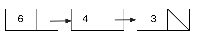
And here is a possible implementation of the list in PRIMP:
| (const EMPTY 0) |
| (data NODE3 6 NODE2) |
| (data NODE2 4 NODE1) |
| (data NODE1 3 EMPTY) |
Note the convention that 0 is not a valid address for data. Note also that the order and position of the data statements is not important. They can be widely separated in memory and still define the same list. This demonstrates the source of some of the power and flexibility of lists. But it does require more care in the implementation than arrays did.
The following PRIMP code will add up the numbers in a list. Here P is a pointer that is mutated to point to successive cons cells. If it is pointing to a cons cell, adding one to it gives the address of a location of memory in which is stored a pointer to the next cons cell (that is, the address of the next cons cell). We do this addition with an indexed operand.
| (move P LIST) |
| (move SUM 0) |
| (label LOOP) |
| (eq TMP0 P EMPTY) |
| (branch TMP0 DONE) |
| (add SUM SUM P) |
| (move P (1 P)) |
| (jump LOOP) |
| (label DONE) |
In this example, recursion is not necessary, as a loop will suffice. An example where recursion helps is printing the list in reverse order. Here’s Racket code for this task. Note that the code is not tail-recursive, so it is not so easy to convert it to a loop.
| (define (print-rev lst) |
| (unless (empty? lst) |
| (print-rev (rest lst)) |
| (display (first lst)))) |
You might try to accomplish this task without recursion in PRIMP, or by using tail recursion in Racket (the above example is not tail-recursive).
The above PRIMP code works with a list that exists as data in the program. What about creating new lists at run time?
We need a source of new cons cells. Here is one strategy for managing this. Define a large chunk of memory with an "allocation pointer" to the first location. This large chunk of memory is typically called the heap (an unfortunately overused word, as there is a completely different data structure called a heap discussed in FDS).
When we need a new cons, we use the two consecutive locations pointed to by the allocation pointer (and add two to it so that it points at unused memory again). In effect, we treat the heap like a stack, except that we never pop.
What happens when all the memory in the heap gets used up? We might need cons cells for intermediate results, but not need them for very long. Cells that are not needed any more can be freed. For instance, suppose we mutate the list above so that it looks like this:
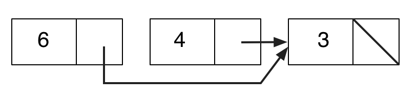
The cell that used to be the second in the list is no longer pointed to by anything, and it can be freed.
Here is one strategy for freeing up unused cons cells. We keep a free list (initially empty). When a cons is not needed any more, we add it to the free list. We change the allocation strategy described briefly above so that we first try to allocate from the free list if it is non-empty. If it is empty, then we allocate from unused memory.
But how do we know that a cons cell is no longer needed? The simplest implementation requires programmers to explicitly free memory. This is not only an additional cognitive burden (requiring the programmer to constantly think about what actions might be resulting in unreachable cons cells, and carefully preserving at least one pointer to them so that they can be freed) but leads to memory leaks if done incorrectly. The alternative is automatic garbage collection, which will be discussed later.
This strategy only works if all we want to allocate are cons cells. What about asking for chunks of memory of different sizes, to use for structures and vectors? This complicates both allocation and de-allocation strategies. Again, we will put off discussion until later.
Our implementation only handles lists of integers. What if we wanted lists containing lists (S-expressions)? We cannot tell the difference between a natural number in the first field of a cons cell and a pointer in this field, because pointers are memory addresses, and any natural number (up to the size of memory) is valid.
One approach is to represent a cons cell by three memory locations instead of two. The additional location holds a type tag for the "first" field.
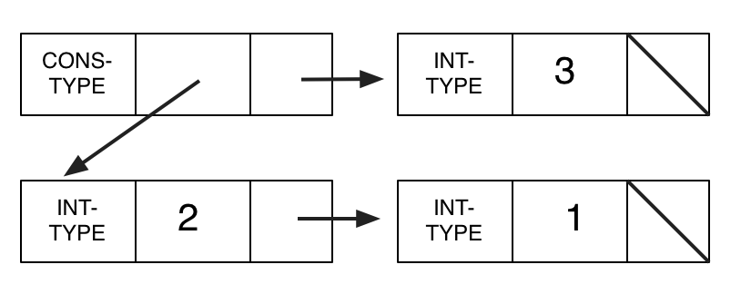
Here is an implementation of the above example in PRIMP.
| (const INT-TYPE 0) |
| (const CONS-TYPE 1) |
| (data NODE2 CONS-TYPE NODE3 NODE1) |
| (data NODE1 INT-TYPE 3 EMPTY) |
| (data NODE3 INT-TYPE 2 NODE4) |
| (data NODE4 INT-TYPE 1 EMPTY) |
A more general approach is to tag all values with their type. This is what Racket does (with some optimizations). The example above might look more like this:
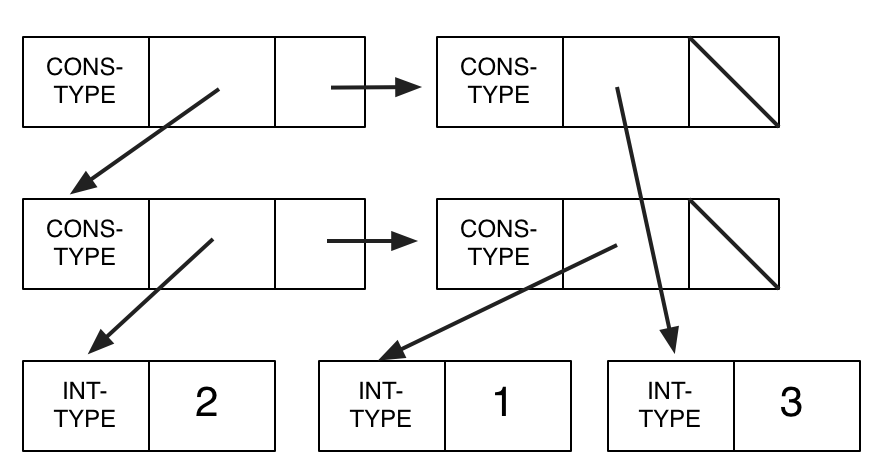
I’ll discuss these ideas in a little more detail later. In the next chapter, we move a level further down, by revealing more details of actual hardware, and discussing the design of a simplified version of an actual machine language and its assembler version.
Exercise 17: Add lists to one of the interpreters you wrote for earlier exercises. \(\blacksquare\)