7 Control
\(\newcommand{\la}{\lambda} \newcommand{\Ga}{\Gamma} \newcommand{\ra}{\rightarrow} \newcommand{\Ra}{\Rightarrow} \newcommand{\La}{\Leftarrow} \newcommand{\tl}{\triangleleft} \newcommand{\ir}[3]{\displaystyle\frac{#2}{#3}~{\textstyle #1}}\)
My goal in this chapter is to sketch how to create a Faux Racket interpreter suitable for implementation in a conventional imperative language like C or SIMP-F. Recursion is not heavily used in such languages; loops are preferred. As a result, their implementations tend to have a small stack and to not optimize tail recursion. As discussed at the end of the previous chapter, we can convert a tail-recursive function to a loop, so if our interpreter written in Racket is tail-recursive, we can more easily translate it into an imperative language. Another goal is to make sure that stack usage does not grow while the interpreter is interpreting a program that is itself tail-recursive.
Although earlier we focussed on big-step interpreters, it turns out that a small-step interpreter is better suited for this conversion. A big-step interpreter often has to do recursion on more than one subtree of the AST (for example, when interpreting an arithmetic expression, recursion is done to compute the value of both operands).
In contrast, the top level of the small-step interpreter repeatedly applies a function that takes one step, so it is tail-recursive. What about the one-step function? It first locates the subexpression eligible for rewriting (this is often called the redex in the technical literature). This only involves one recursion for each case, since we can identify which child subtree of the current AST contains the redex.
Once the redex is located, the one-step function rewrites it and produces the result. We also have to make the rewriting tail-recursive. The hardest case is when the redex is the application of a lambda to a value. This requires substitution in the body of the lambda. Substitution is not tail-recursive, and it is also inefficient. We know how to deal with this by maintaining an environment of name-value pairs to defer substitution.
Once the rewriting is handled, the one-step function produces the new AST. But on the return from the recursion, the returned value is put into an AST node with the parts of the tree uninvolved in the recursion. That is, the unchanged parts of the AST are reconstructed on the way back from the recursion. So this is not tail-recursive, as work is done after the recursion. But it’s close.
We also have the inefficiency of starting from the top of the AST every time we try to find the redex. Intuitively, the next redex is usually somewhere close by. The solution to this is the same as the way to complete the conversion to tail recursion. It is a data structure known as a zipper, which maintains a position in a list or tree and allows efficient "backing up". (The name was bestowed by Gérard Huet when he described it in 1997, though he said at the time that it was a known "folklore" technique.)
7.1 Zippers
Consider the following trace from earlier in the course.
| (append (cons 1 (cons 2 (cons 3 empty))) |
| (cons 4 (cons 5 empty))) |
| =>* (cons 1 (append (cons 2 (cons 3 empty)) |
| (cons 4 (cons 5 empty)))) |
| =>* (cons 1 (cons 2 (append (cons 3 empty) |
| (cons 4 (cons 5 empty))))) |
| =>* (cons 1 |
| (cons 2 |
| (cons 3 (append empty |
| (cons 4 (cons 5 empty)))))) |
| =>* (cons 1 (cons 2 (cons 3 (cons 4 (cons 5 empty))))) |
As the recursion proceeds, the redex appears deeper and deeper inside the fixed part of the eventual result. In this case the new redex appears inside the result of the rewrite, so it is not hard to "descend" to the right spot.
But how would we "ascend" once the current redex becomes a value? In the above example, this only happens when the final result is computed, but consider the example of a complex arithmetic expression. The first step would replace the leftmost node with two leaves by a single number, so some sort of backing up would be needed.
Let’s consider the same problem of navigating in a data structure, but with a list instead of a tree. We won’t need the list version in our application, but it’s easier to see how it works, and to generalize to a tree.
We want to maintain a notion of a "current element" or position, with operations such as moving back and forth, possibly modifying the current element, deleting the current element, or adding a new element before the current one. The goal is to do these operations in constant time.
One imperative solution uses a doubly-linked list with a current element pointer, as described in IYMLC.
With this representation, moving back and forth is simple, but setting the doubly-linked list up, modification, insertion, and and deletion all make heavy use of mutation.
Can we do this with a purely-functional data structure?
Yes. We can use a structure containing two lists, representing "ahead" and "seen" respectively. But to be able to generalize later, I’ll represent the "seen" list by a new data type of contexts, reminiscent of the development in Part I where I described lists using structures before introducing Racket lists.
| (struct MT ()) |
| (struct F (elt rst)) |
| (struct CList (ahead seen)) |
Here the F constructor plays the role of "cons", and the MT constructor plays the role of "empty". "F" stands for "forward", and we’ll see why it’s called that shortly.
Suppose our example list is '(1 2 3 4). We represent this as (Clist '(1 2 3 4) (MT)). Moving forward results in (Clist '(2 3 4) (F 1 (MT))). Moving forward again results in (Clist '(3 4) (F 2 (F 1 (MT)))).
The key insight is that keeping the "seen" list in the order it would be encountered while moving backwards (the most recently seen item is at the front of the data structure) facilitates backing up in constant time.
Exercise 24: Write Racket code for the move-forward, move-backward, modify-here, insert-here, and delete-this operations on Clists. Each operation should run in constant time. \(\blacksquare\)
We could have just used regular lists for the "seen" list, but as I mentioned, it’s easier to generalize our own structures to the tree case. The same technique will work for moving about in a tree. The difference is that the context must include not only the information at the node moved forward from but also into what subtree and how to move back. For example, in a binary tree, we need to be able to tell from the context whether the last move forward descended left or right, and what the subtree forming the other branch was.
| (struct BTnode (elt lft rgt)) |
| (struct L (elt bt ct)) |
| (struct R (elt bt ct)) |
| (struct CBTree (bt cxt)) |
Note that the context is still "list-like", in that each data constructor only has one recursive field. "L" stands for "left" and "R" for "right", the directions we can go to descend; we need this information to back up. Now you can understand why, in the list case, I used "F" for forward.
If we have (CBTree (BTnode a l r) c) and wish to descend left, the result is (CBTree l (L a r c)), but if we wish to descend right, the result is (CBTree r (R a l c)).
Exercise 25: Write Racket code for the move-left, move-right, move-back, and modification functions for CBTrees. Each function should run in constant time. \(\blacksquare\)
7.2 A continuation-passing interpreter
In the special case of the AST for an interpreter, the context is called a continuation. We create a structure for each possible way of moving forward in the AST that is useful for the interpreter, and store whatever information is necessary to back up.
| (struct MT ()) |
| (struct AppL (ast cont)) |
| (struct AppR (val cont)) |
| (struct BinOpL (op ast cont)) |
| (struct BinOpR (op val cont)) |
Because our goal is a tail-recursive interpreter, we don’t need to wrap the continuation together with the AST (the current expression) in a pair, as in the abstract examples in the previous section. We can simply add the continuation as a new parameter (the current expression is already a parameter).
Our interpreter interp will now consume two arguments, an AST, and a continuation. If the root of the AST is a Bin or App, it descends. In these two cases, while evaluating subexpressions that are arguments, the continuation grows.
In the remaining cases, the AST represents a value. The interpreter ascends by "applying" the continuation to the value. For clarity, we split this out into a separate function, apply-cont, which consumes a continuation and a value, and produces a value. This function is mutually recursive with the interpreter function. For example, if apply-cont is applied to (BinOpL op y k) and v, it applies interp to y and (BinOpR op v k). But if apply-cont is applied to (BinOpR op v1 k) and v2, it figures out the result v of applying the operator op to v1 and v2, and recursively applies itself (apply-cont) to k and v.
If you work out all the cases (which you should do), you will see that in some of them (such as the first one above), when evaluating subexpressions, the continuation in the recursive application changes (but does not get "longer"). In other cases, such as applying a primitive operation or function, the continuation in the recursive application does not change. This code is tail-recursive, so we can put it into a loop.
Where is the stack? The continuation plays that role. But the continuation grows when evaluating subexpressions, not when applying functions. In other words, if the interpreted program is tail-recursive, the interpreter will not use extra control space.
This is not the result of using continuations. It was true for the Stepper also (though less obvious). We can see the effect when stepping through the tail-recursive implementation of factorial or Fibonacci; the size of the expression does not grow.
7.3 Adding back environments
We are not finished. Substitution is expensive and it is not tail-recursive. But we know how to handle that. As before, we add an environment parameter to our interpreter, handling name-value bindings. Again, as before, a closure is created from a Fun expression when evaluated, by saving the environment. Environments also need to be saved in some continuations.
It is possible for recursive functions producing functions to create arbitrarily large environments, pointlessly. This can be fixed when a closure is created. The associated environment should contain only bindings for the free variables of the body of the function.
Now that we have made the interpreter fully tail-recursive, it is relatively simple to add mutation to the interpreter as we did earlier, with the use of a store. Threading the store through the computation is a lot easier than before; it is just another accumulative parameter in interp.
Whether or not we do this, we now have two mutually-recursive functions, interp and apply-cont, both tail-recursive. Our interpreter is now ready for translation into an imperative language.
Exercise 26: Complete the Racket implementation of the Faux Racket interpreter that is continuation-passing and environment-passing. \(\blacksquare\)
Exercise 27: Add set and boxes to your answer to the previous exercise. Also add rec as in exercise 5, but this time don’t use mutation in Racket; instead, just desugar it to other Faux Racket constructs, as was done with let earlier. \(\blacksquare\)
7.4 Trampolining
There are two ways we can proceed.
Idea 1 is to merge the two mutually-recursive functions into one loop, with parameters becoming loop variables.
Idea 2 preserves more structure, and is generally applicable to a larger collection of mutually-recursive functions. It is known as trampolining.
We write a trampoline function, which calls the first tail-recursive function to start the computation. Instead of that function calling another function in tail position, it returns a "bounce" to the trampoline. The "bounce" is a data structure that contains the information needed for the trampoline to call the next tail-recursive function (name and arguments).
This results in bounded stack depth, even when implemented in C. We illustrate with a fragment of a Racket implementation, which is clearer (though unnecessary, as Racket optimizes tail calls).
| (struct bounce (function args)) |
| (define (trampoline x) |
| (if (bounce? x) |
| (trampoline |
| (apply (bounce-function x) |
| (bounce-args x))) |
| x)) |
Every use of (interp x cont env) is replaced by (bounce interp (list x cont env)). We start the process off at the top level with (trampoline (bounce interp (list x mt-cont mt-env))) (where x is the expression to be interpreted). We cannot directly translate this Racket implementation into an imperative language, because we typically don’t have functions as values or apply in such languages.
There are a number of substitutes that will work. One for the C language involves function pointers, which have to point to functions known at compile time. A function pointer type includes the number and type of each argument, so the translation is not direct.
A more general (and perhaps easier) approach is to put arguments into global variables and make the mutually-recursive functions have no formal parameters. Each function will take its arguments from the global variables when called, put the arguments for the tail call into global variables, and return (to the trampoline function) a function pointer to the next function to be called. This reduces a function application to a jump, like in PRIMP and FIST (this is also possible in C via the discouraged goto statement).
7.5 Garbage collection
The trampolined interpreter written in Racket, or another functional programming language, relies on unused memory being reclaimed automatically at run time. Where does this need to happen in a translation to C or another imperative language that does not automatically do this?
Continuation structures
Environment structures
Cons cells used in environments
Cons cells used in interpreted language (if implemented)
It’s not obvious when to free any of these. Implementing closures means that environments no longer behave like stacks (last allocated / first deallocated).
We need to implement some form of garbage collection to reclaim unused heap memory. Here, we will briefly discuss the concepts behind three classic algorithms. The topic remains the subject of active research, and many popular modern programming languages use garbage collection.
7.5.1 Reference counting
The first technique is called reference counting.
In every chunk of heap-allocated memory, we maintain a "reference count" of the number of pointers that point to it. This count starts at one when the chunk is allocated, and is incremented each time we copy a pointer.
frees a chunk containing a pointer
returns from a function having a local pointer variable pointing to the chunk
mutates a pointer variable that was pointing to the chunk
When the reference count is decremented to zero, the chunk is freed. This may trigger further freeing.
One advantage of this method as compared to the other methods we’ll discuss is that it can be done on the fly, instead of having to stop and do a lot of work. A cascade of freeing, as might happen if the reference count of the head of a long list reaches zero, can still happen, depending on the code.
One disadvantage is that programmer effort is required to identify increment and decrement points all throughout the code. In the case of a new implementation of a programming language, support can be built into the compiler or interpreter.
Another disadvantage is that reference counting does not work properly when there are cycles of pointers.
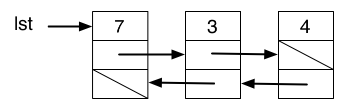
Here we have shown the reference counts and pointers, not other data. If the pointer lst is mutated, then the reference count of the node it is pointing to drops to zero and the node is freed. But the reference count of the next node drops to one, and the others stay at one, so they are not freed, even though they are no longer accessible.
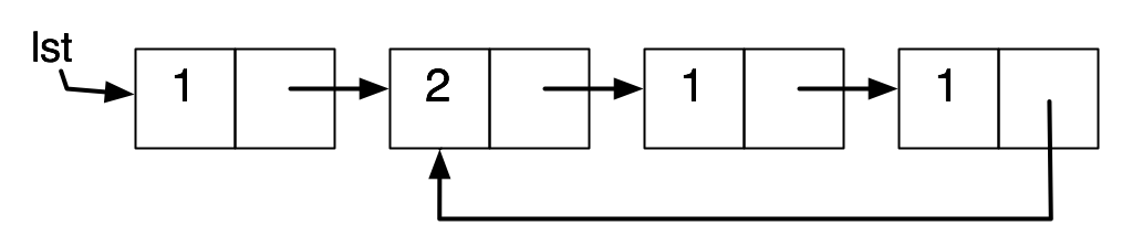
This is less of a problem if the interpreted language does not support mutation. The data structures created by the interpreted code cannot have cycles in them.
But we introduced a cycle in environments containing bindings for recursive functions. Here is an example where f is bound to a closure containing an environment in which f is bound.
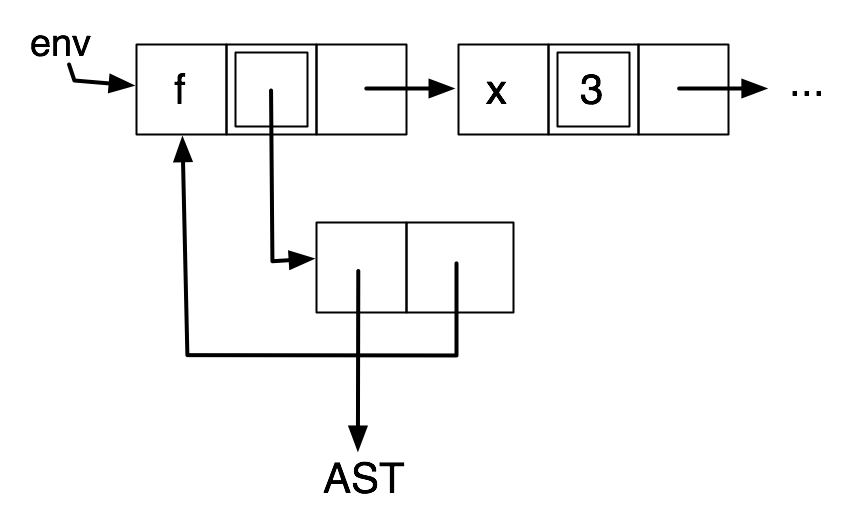
This cannot be avoided without much effort. But it is a special case that can be detected and handled.
Or: we can use reference counting until memory runs out, then reclaim the circular structures using one of the next methods.
7.5.2 Mark-and-sweep
The second technique is called mark-and-sweep. It is described in McCarthy’s original paper on Lisp (1959).
The set of active heap chunks can be found at any point by a "graph reachability" search from the current environment and continuation. These active heap chunks can be "marked" in the course of the search (by setting a dedicated bit somewhere in the chunk). A subsequent "sweep" through all of heap memory can reclaim unused chunks (those that have not been marked and are therefore inaccessible).
One advantage of this method is that it can be mostly buried in the allocation wrapper function. A mark-and-sweep pass occurs when an allocation is attempted and there is no more free memory. One disadvantage is that it may cause a long pause while memory is reclaimed. Another is that the marking may use a lot of stack memory itself, being a recursive algorithm.
Another disadvantage of both reference counting and mark-and-sweep is that they do not address fragmentation of memory. Fragmentation is the situation where lots of small allocated blocks are scattered through memory preventing consolidation of free chunks into larger ones.
This is not an issue if only one size of chunk is being allocated, as in our earlier discussion of implementing alloc/free for cons cells using an allocation pointer and free list. In effect, all of memory is divided into cons cells, and there is no real fragmentation.
But what if we want to allocate different-sized structures? We could keep a separate free list for each size. But balancing between sizes becomes difficult. If this is driven by the program, it may initially use lots of memory up with one size, and then start asking for another. If it is predetermined, then the program may run out of one size when there is plenty of memory free (but earmarked for another size).
One common solution to this is called the buddy system. We start with blocks of some small size \(k\). We pair them up into blocks of size \(2k\), pair those up, and so on. We maintain a free list of each block size (initially just one block of the largest size).
When an allocation request arrives, we try to satisfy it by the next largest block size. If that size is not available, but the next larger one is, we can split it in two, put one on the free list, and give one to the request. If the next larger size is not available, we go up to the first size that is available, splitting larger blocks up as needed.
When the program frees memory, we try to repeatedly merge the freed block with "buddies" to make the largest free block we can. That is, if the newly-freed block is the buddy of an earlier freed block, we take the earlier block off its free list, merge the two, check if the buddy of the merged block is free, merge with that (and remove it from its free list), and so on. Eventually we get to a free block that cannot be merged with its buddy, and we put that on the appropriate free list.
The buddy system reduces but does not eliminate fragmentation. It’s possible for small free blocks to be intermixed with small allocated blocks in such a way that a larger allocation request cannot be satisfied. It also may waste memory (since typically more memory is allocated than needed), and is likely overkill for a language where mostly small chunks are allocated (say, a language with cons and struct but not vector).
7.5.3 Copying garbage collection
The third technique addresses the issues above. It is called copying garbage collection, and the idea is originally due to Cheney.
Copying garbage collection divides memory into two chunks: working and free. We use the allocation pointer and free list method to allocate from working memory, until it is exhausted.
At this point, the memory still used in the working memory half is copied into the free memory half, in a manner we describe below, and the roles of the two halves are then switched. The copying from working memory to free memory is done by an ingenious algorithm that does not require recursion, and uses only two additional pointers into free memory: free and scan.
The free pointer is an allocation pointer, pointing to the next usable location in free memory. The scan pointer lags behind. Between the two are chunks that have been copied but still contain their old pointer values (pointing into working memory).
To start with, both free and scan point to the start of free memory. One chunk (from which all other chunks would be accessible by graph reachability) is copied from working memory into free memory (moving the free pointer).
When a chunk is copied, it is marked in working memory, and (important) its first pointer is changed to point to the copy in free memory. The main loop of the algorithm moves scan to the next chunk in free memory, and checks all its pointers.
Any pointer that points to another chunk of working memory not copied yet results in that chunk being marked and copied (free moves). Any pointer that points to a copied chunk is updated with the new location of that chunk (stored in the old chunk).
When scan catches up with free again, all reachable chunks in working memory have been copied to free memory. At this point, there are no "holes" in free memory.
This basic idea can be extended to "generational" garbage collectors, which take advantage of common allocation/deallocation patterns (many short-lived objects, some long-lived ones). Another interesting topic which I will not cover is "real-time" garbage collectors, which avoid the need to pause computation for significant periods of time. This remains an active area of both research and intense engineering focus.
7.6 What’s next?
The next chapter is optional reading, so this is a good time to pause and suggest some paths forward. If you want to learn more about imperative programming, I suggest that you spend a small amount of time learning some C without getting too deep into its quirks and pecularities, perhaps by using IYMLC or the textbook it suggests. After that, you might spend time with the Rust programming language, which offers a modern and principled approach to low-level systems programming.
If you want to learn more about functional programming with effects, my flâneries FDS (using OCaml) and LACI (using Racket, Agda, and Coq) are suitable, as well as their sources and the sources I cite in the Handouts chapter.