2 Effects in Racket
\(\newcommand{\la}{\lambda} \newcommand{\Ga}{\Gamma} \newcommand{\ra}{\rightarrow} \newcommand{\Ra}{\Rightarrow} \newcommand{\La}{\Leftarrow} \newcommand{\tl}{\triangleleft} \newcommand{\ir}[3]{\displaystyle\frac{#2}{#3}~{\textstyle #1}}\)
In one of the courses based on the material I presented in Part I, I moved to full Racket at the end of the material on generative recursion. Part of that was to spread out the transition so that everything did not hit in the first week or two of a new term, but there are features in full Racket that improve expressivity even if one is not considering imperative features (as was the case for the rest of the material in that course, and the rest of the material in Part I).
I will maintain this separation here, because I think it is important. First, we will move to full Racket without considering the features that will dominate Part II. Those I will start introducing gradually, after the transition.
2.1 Moving to full Racket
Although we are moving away from the teaching languages, we will use only a small fraction of the features available in full Racket. The whole diverse Racket ecosystem is best explored slowly, at one’s leisure. The move is handled by the same Choose Language menu item we have been using, with the choice "The Racket language". This actually lets us choose from among a family of languages, and the one we will be using is indicated in the program by putting #lang racket on the first line.
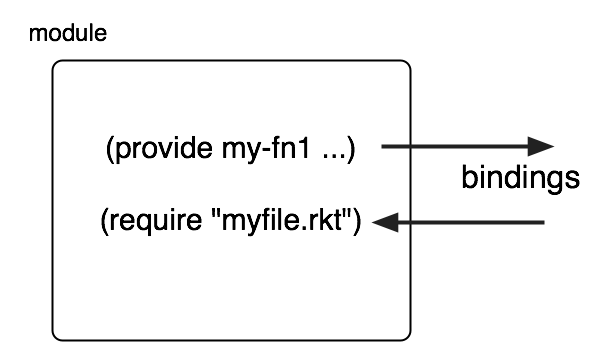
That first line is syntactic sugar that has the effect of wrapping the whole program in a module expression. Modules are an effective mechanism for distributing a Racket program among multiple files, as well as handling some problems associated with the top-to-bottom semantics we have been using. Racket’s module system provides forms for exporting bindings (provide) and importing bindings (require). Both of these have many options, some of which we will explore later.
The teaching languages are not strict subsets of full Racket, and you will have to make some adjustments. The Stepper is gone, replaced by a more complicated Debug button (which I personally have never used, so you needn’t worry about it for now). check-expect is not automatically predefined, and its nice user interface is gone. The following code sequence gets back some of the functionality. Note the use of require to load bindings for useful functions (in this case, the ones that let the programmer specify and run tests).
| (require test-engine/racket-tests) |
| ... |
| (check-expect ...) |
| ... |
| (test) |
The module required in the above code loads the core testing mechanism that is used in the teaching languages. This is good for small programs such as might be written for exercises here, but is not adequate for larger programs. Racket has a more scalable "unit testing" mechanism called RackUnit. The simplest use looks like this:
| (require rackunit) |
| ... |
| (check-equal ...) |
RackUnit has a number of test functions, as well as the ability to group tests into cases (where a failure stops the rest of the tests in the case) and into suites which can be run or not depending on circumstances. You might look into this if you use Racket for projects of your own.
Structures are opaque by default. This is useful for abstract data types which do not leak details of their implementation. However, quite often, we don’t want this to happen; we want to see inside structures. We can make the structures transparent by using a keyword argument.
(define-struct posn (x y) #:transparent)
Here the keyword #:transparent merely turns on a capability, but keyword arguments for forms and functions can allow the specification of associated values. Keyword arguments are not positional and can have defaults, so they can be omitted. Rather than describe the full general mechanism, I’ll just use keyword arguments occasionally when they prove useful.
We can use the struct form instead of define-struct. Both of these create a constructor function with the same name as the structure. define-struct also creates the "make-" constructor familiar to us from the teaching languages.
| (struct point (x y) #:transparent) |
| (point 2 3) |
The teaching languages enforce the restriction that the second argument of cons should be a list, that is, empty or another cons. This is not enforced in Racket (or in standard Scheme). (cons 1 2) is a legal expression, producing what is sometimes called a "dotted pair", which displays as (1 . 2). I will not use dotted pairs in this flânerie; I mention them here only so that you recognize what you have done wrong if you make a mistake and see a dot in what you thought was a list value.
Full Racket permits internal definitions in a "body" of code, for instance, in the body of a defined function, lambda, or cond answer. We will most often use these as a shorter form of local.
| (define (f x) |
| (define (g x) (- x 3)) |
| (sqr (g x))) |
The leap from the teaching languages to full Racket is large, and there is no safety net. It is too easy to make mistakes which result in legal programs. Here is a small example where the programmer has temporarily forgotten to use prefix notation for addition.
| (define (len lst) |
| (cond |
| [(empty? lst) 0] |
| [else 1 + (len (rest lst))])) |
This code will not run in the teaching languages, but it is legal in full Racket. This function produces 0 for all lists. We will see why shortly.
In preparation for what follows, we need a way of evaluating several expressions but only producing the value of the last one. This is provided by the begin form. Here is the grammar rule:
| exp | = | (begin exp exp ...) |
And here are the rewrite rules:
| (begin val exp ...) => (begin exp ...) |
| (begin exp) => exp |
This form would be useless in the purely-functional teaching languages. It is used with expressions that have effects (they do things in addition to producing a value). Effects are sometimes called side effects. We have already been using effects, though we didn’t characterize them as such. When a top-level expression in a program is evaluated, the resulting value is printed in the Interactions window. That is an effect. One of the ways we can extend this particular effect is by a mechanism that permits this for expressions that are not at the top level.
In full Racket, there is an implicit begin at several points. For example: in the body of functions, lambda, and local, and in the answers of cond. This explains the behaviour of the incorrect implementation of len above. The answer for the else is treated as three separate expressions; the first two are evaluated (very quickly, since they are the constant 1 and the constant built-in function +) and the value of the answer is the value of the recursive call. This is why the base value 0 is always produced.
The implicit begin shortens code and reduces indentation, at the cost of allowing a wider range of errors. This makes more careful development and testing even more important than with the teaching languages.
2.2 Quasiquotation and pattern matching
The Beginning Student with List Abbreviations language (BSL+) gave us the ability to specify nested lists using an apostrophe (close single quote), as with '(* (+ 1 2) (+ 3 4)). In '(1 x 2), the mention of x becomes the symbol 'x. If there were a variable x that we wished to refer to instead, we would need to use the list form, as in (list 1 x 2).
Quasiquotation (also present in BSL+, though I didn’t mention it earlier) extends the convenience of list quotation to this situation. Quasiquote (usually abbreviated with an open single quote, as in `(1 2 3), works like quote, but it allows "escapes" to embed arbitrary Racket expressions. If such escapes are not used, it behaves like quote.
| (define x 3) |
| `(a b x) |
| => '(a b x) |
Escapes within a quasiquote expression are handled by unquote (abbreviated with a comma):
| (define x 3) |
| `(a b ,x) |
| => '(a b 3) |
Here I have used the Racket expression x, which in the given context will evaluate to 3. But we can replace x with an arbitrary Racket expression.
| (define x 3) |
| (define y '(c d)) |
| `(a b ,(+ 2 x)) |
| => '(a b 5) |
| `(a b ,y) |
| => '(a b (c d)) |
At times we want to evaluate a Racket expression with a list value, but not just put the list value into the quasiquoted expression. Instead, we want to "splice" the computed list elements in. This is accomplished with unquote-splicing (abbreviated with a comma and at-sign):
| (define x '(c d)) |
| `(a b ,@x) |
| => '(a b c d) |
Quasiquotation improves expressivity when constructing complex values. The next feature I want to discuss improves expressivity when deconstructing complex values. It’s not predefined in the teaching languages, but it can be imported into Intermediate Student and higher using require. In one course, I did this as early as the end of the Lists chapter, because it was so useful.
The match form resembles cond, but makes use of pattern matching. There is an initial expression which is reduced to a value, and the question/answer pairs of cond are replaced by pattern/answer pairs. A pattern can have literal parts but also can bind variables for use in the corresponding answers.
| (match exp |
| [pattern answer] |
| ...) |
Patterns have a recursive definition. An identifier by itself is a primitive pattern that matches any value; that value is bound to that identifier. In the code below, the pattern y matches the value of x (regardless of what it is) and, in the answer, the variable y is bound to that value.
| (define (f x) |
| (match x |
| [y (+ 3 y)])) |
| (f 2) => 5 |
| (f 5) => 8 |
Numbers and strings are primitive patterns, matching their values. You can think of these as specifying literal parts of a compound pattern.
| (define (f x) |
| (match x |
| [3 "three"] |
| ["four" 4] |
| [y false])) |
| (f 3) => "three" |
| (f "four") => 4 |
| (f 5) => false |
We can form a compound pattern by applying the pattern element list to a sequence of several patterns. In the example below, the pattern (list x y) matches a two-element list value, and binds x to the first element of the list and y to the second element of the list. Notice the local rebinding of x. In the answer (+ x y), x does not refer to the argument of f, but to the first element of that argument, if it is a two-element list.
| (define (f x) |
| (match x |
| [(list x y) (+ x y)] |
| [(list x y rst ...) |
| (list (- x y) rst)] |
| [(list 1) false])) |
| (f '(1 2)) => 3 |
| (f '(1 2 3 4)) => '(-1 (3 4)) |
| (f '(1)) => false |
The above example also shows how the ellipsis (...) can be used with an identifier to bind that to the rest of the list, allowing matching against lists of arbitrary length. Here the ellipsis is not standing in for missing code; it is an actual part of the pattern.
Identifiers can be repeated in a pattern, indicating a repetition of a value in whatever matches. In the example below, the list '(1 3 2) would not match any of the patterns, and a run-time error would result if g was applied to it.
| (define (g x) |
| (match x |
| [(list x y x) (+ x y)] |
| [(list (list x y) z) (- x z)] |
| ['(1 (2 3)) true])) |
| (g '(1 3 1)) => 4 |
| (g '((4 8) 3)) => 1 |
| (g '(1 (2 3))) => true |
In patterns, cons can be used as well as list to construct patterns matching list values. The underscore ("_") can be used as a pattern to indicate the presence of a value that need not be given a name. Structures can be matched by using the keyword struct, followed by the name of the structure, followed by a parenthesized list of patterns, one for each field of the structure. The keyword struct can also be omitted.
| (define (h x) |
| (match x |
| [(cons 1 (list y z)) (+ y z)] |
| [(list p _) (sqr p)] |
| [(struct posn (p q)) |
| (list p q)])) |
| (h '(1 2 3)) => 5 |
| (h '(2 3)) => 4 |
| (h (make-posn 7 8)) => (list 7 8) |
We saw above that while quote (abbreviated as single close quote) can be used to construct list values, quasiquote (abbreviated as single open quote) also permits this, with the added advantage that within a quasiquoted expression, unquote (abbreviated with a comma) escapes to regular Racket expressions.
Quasiquote plays a similar role in patterns, except that here, unquote escapes to patterns.
| (define (h x) |
| (match x |
| [`(1 ,y ,z) (+ y z)] |
| [`(,(struct posn (p q)) ,r) |
| (list p q r)] |
| [`(,p ,_) (sqr p)])) |
| (h '(1 2 3)) => 5 |
| (h (list (make-posn 7 8) 9)) |
| => '(7 8 9) |
| (h ('3 4)) => 9 |
We will find pattern matching very useful in writing readable code to deal with complex data structures. As an example we will return to later, consider the small interpreter for arithmetic expressions we developed in the Lists chapter of Part I.
| (define (interp exp) |
| (cond |
| [(number? exp) exp] |
| [(symbol=? (first exp) '*) |
| (* (interp (second exp)) |
| (interp (third exp)))] |
| [(symbol=? (first exp) '+) |
| (+ (interp (second exp)) |
| (interp (third exp)))])) |
Here is a version of it using match.
| (define (interp exp) |
| (match exp |
| [(? number? n) n] |
| [`(* ,x ,y) (* x y)] |
| [`(+ ,x ,y) (+ x y)])) |
The first pattern, using ?, applies the predicate number? to the value being matched, and if it produces true, matches the pattern n against it; the pattern n matches anything, and binds n to the result for use in the answer. The point here is that the version of interp using match is made more readable by pattern-matching using quasiquote patterns.
As with cond answers, match answers also have an implicit begin. There are many other features of match, and some related forms that offer useful variations. I will introduce these as needed, but you are welcome to look at the Racket documentation and start using them in your own code (warning: the documentation for full Racket is generally quite good, but is not written for beginners, and can be hard to understand at times).
Unlike with most other Racket features I have introduced, I won’t give full rewriting rules for match. Intuitively, a match expression can be expanded into an often much larger statement using just if or cond. In fact, this is literally what happens, since match is implemented using macros.
Exercise 0: Give rewriting rules for as much of match as you care to specify. \(\blacksquare\)
2.3 The memory model
We can introduce interaction (input, output) and some forms of mutation (changing name/value bindings) without too much change to the substitution model that we used in Part I, though the model does become more elaborate. Sometimes the details are messy but straightforward, and I will say so, and not write them out. Some other forms of mutation (in fact, everything we learn about in this flânerie) can still be handled within the substitution model, but they render the model less effective as a tool for understanding or tracing programs. If the details are messy and also present conceptual challenges or problems that need to be overcome, I will sketch as many of the details as are necessary to make the ideas clear. In other words, I will try to adopt a more practical or pragmatic approach, without entirely abandoning the model for the treacherous grounds of "intuitive understanding".
Some of the details are better described in a model that more closely resembles the actual workings of a computer. That model is called the memory model, and it explains computation by detailing how information is stored and modified. Using only the memory model, it is difficult to explain some of the things that were easy to deal with in the substitution model. Consequently, we will use a combination of the substitution model and the memory model to handle concepts in Part II.
Memory can be viewed as a sequence of boxes indexed by natural numbers, each one containing a fixed-size number. We will eventually use the model of memory shown in the picture below, which is an approximation to actual hardware, but still simplifies it by omitting many important details.

Although current architectures are 64-bit, the essential details are the same at the conceptual level we will be working at, and using only 32 bits avoids having to write out some long numbers. We will not be using the memory model for some time, but it is our eventual destination, and influences the path to that destination, so it is worth keeping it in mind as we proceed.
2.4 Output
Recall that the substitution model shows how to reduce a program (a sequence of definitions and expressions) to a sequence of definitions and values. The values are then printed, one to a line, in the Interactions window.
Racket allows values to be printed at other points during the computation, and they can also be stored in files. In order to model this, we have to be a bit more precise about the substitution model. We treat what appears in the Interactions window as an unbounded sequence of characters that we call the output sequence. A function that performs output simply appends characters to the end of this sequence.
In the Functional Abstraction chapter of Part I, I briefly discussed the fact that Racket strings can be considered as sequences of characters, but we did not spend much time treating strings as compound data. Just as we view the word "cat" as being made up of the three characters ’c’, ’a’, and ’t’, we can view the Racket string "cat" as being made up of three characters. But we have to convert the string to another type of value in order to manipulate those characters. For instance, the result of evaluating (string->list "cat") is the list '(#\c #\a #\t). The character ’c’ is represented in Racket by the value #\c.
Previously, when discussing computation in Racket using the substitution model, we just reduced or rewrote a program \(\pi\), resulting in a sequence of equivalent programs \(\pi_0\Rightarrow \pi_1 \Rightarrow \ldots \pi_n\). Now we must add a parallel rewriting of the output sequence: \(\omega_0\Rightarrow \omega_1 \Rightarrow \ldots \omega_n\). Mathematically, it is simpler to combine the two into a single sequence: \((\pi_0, \omega_0)\Rightarrow (\pi_1,\omega_1) \Rightarrow \ldots (\pi_n,\omega_n)\). Conceptually, this is straightforward, but when we get more precise, there are some complications having to do with the fact that definitions can also be created or rewritten during a computation (we have already seen the creation of new definitions in the rewrite rule for local in Part I). To deal with this, we add a separate component to the tuple consisting of definitions.
In other words, the computational model now maintains and rewrites a tuple \((\pi,\delta,\omega)\), where \(\pi\) is a sequence of definitions and expressions, \(\delta\) is a sequence of definitions of the form (define id val), and \(\omega\) is the output sequence. The initial tuple \((\pi_0,\delta_0,\omega_0)\) has \(\delta\) and \(\omega\) empty.
If the first element of \(\pi\) is a definition of the form (define id exp), then we rewrite exp according to the rules we have worked out so far (and new ones for the new features we will discuss later). This rewriting of a definition might result in characters being appended to the output sequence \(\omega\) as well. Once exp is reduced to val, the definition is removed from \(\pi\) and added to \(\delta\), where it can be looked up for subsequent uses.
If the first element of \(\pi\) is an expression, it is reduced to a value (during which characters may be appended to the output sequence \(\omega\)). The value is then removed from \(\pi\), and the characters of the printed representation of the value are appended to \(\omega\). When \(\pi\) becomes empty, the computation is done.
We refer to the elements that change during the sequence of rewrites (apart from the simplification of expressions in \(\pi\)) as state. Dealing with the consequences of state is going to be our preoccupation in Part II. Currently the only state element in our tuple is the output sequence, and this is relatively innocuous, because future computation does not depend on past changes to the output sequence. The sequence of definitions \(\delta\) is changing during the computation, but each individual definition does not change after it is moved from the program or created as a result of using local, so it is not yet state. Soon we will how definitions can change, affecting future computation, and this will be harder to deal with.
I will now discuss new features which will result in \(\omega\) being appended to during the reduction of an expression (informally, we describe this as some value being "outputted"). There are several different functions that will output the value of an expression (in the examples below I have used a very simple expression, namely a variable such as x).
| (display x) |
| (newline) |
| (write x) |
| (printf "Answers: ~a and ~s\n" x y) |
The display function outputs its argument when it is evaluated. Values that are the result of reducing top-level expressions are printed one to a line, but this is not the case for values displayed using display. If we want to start a new line, we can use the newline function, which appends a special newline character to the output sequence. When displayed in the Interactions window, this has the effect of starting a new line. write acts like display, except that it is more suited to produce data which will later be read by another program. As a brief example, write prints a string using double quotation marks, and display does not.
printf stands for "print formatted". The name is taken from a C function which is one of the first things discussed in my flânerie IYMLC, because C does not have an equivalent to the Interactions window, and without that C function, one cannot get any information from a program. The first argument of printf is a format string with placeholders, which are special points in the string indicated by tildes (~) where the value of another argument is inserted to create the output. There should be exactly as many tilde-indicated placeholders as there are other arguments after the format string. "~a" in a format string produces output like display, and "~s" produces output like write. "\n" in the format string starts a new line. The two characters in the format string, backslash and lower-case n, together represent a single newline character (whose Racket value is #\newline). The format string is just a Racket string value, and this convention for putting a newline character into a string (which is part of a general mechanism for describing special characters within strings) holds for all Racket string values.
The ability to insert the printed representation of a value into a string is quite useful if one is working extensively with strings. The format function works like printf, but it is a pure function with no side effects; it does not output anything, but produces the resulting string.
This suggests the question: what value do the above expressions involving display and write produce?
They produce a special value #<void>. This value has the property that it is not displayed in the Interactions window if it is the result of evaluating a top-level expression in a program, or the result of evaluating an expression typed in at the prompt in the Interactions window.
The value #<void> can also be produced by the expression (void). More generally, void is a function that consumes any number of arguments and produces #<void> (ignoring the arguments). The point of evaluating an application of void (or of display or printf) is the effects from the evaluation of its arguments, so the value produced is not a useful one. An expression that produces only the useless value #<void> is sometimes called a statement, but this term is not really used in Racket; it is used for imperative languages such as C, and I will use the term more when discussing languages that are more imperative than functional.
It is not hard to imagine more elaborate computations that are performed primarily for effects and not for the value produced. The for-each function is an abstract list function that works like map, except that it does not produce a list. It consumes a function f and a list lst, and applies f to each element of lst, but discards the resulting values and produces only #<void>. This is only useful when the application of f has effects. Here is an expression that displays each element of a list, separated by spaces (note the space after the tilde-a in the format string). The value of this entire expression is #<void>.
| (for-each |
| (lambda (x) (printf "~a " x)) |
| lst) |
Like map, for-each can be easily written using structural recursion on the list argument.
| (define (for-each f lst) |
| (cond |
| [(empty? lst) (void)] |
| [else (f (first lst)) |
| (for-each f (rest lst))])) |
In the above example, we could replace cond with if.
| (define (for-each f lst) |
| (if (empty? lst) |
| (void) |
| (begin (f (first lst)) (for-each f (rest lst))))) |
This situation, of conditionally evaluating code that has effects and essentially doing nothing otherwise, is common enough that it has a more readable alternative in Racket, the unless form.
| (define (for-each f lst) |
| (unless (empty? lst) (f (first lst)) (for-each f (rest lst)))) |
The similar when form evaluates its body expressions when the test expression is true (producing the value of the last one), and produces #<void> otherwise.
Instead of the output being sent to the Interactions window, we can choose to accumulate it in a file, using the function with-output-to-file. The first argument is the name of a file. In this example, it is specified as a string, which results in a file being created in the same directory as the program. There are more general mechanisms available that work with the directory or folder structure of the computer. The second argument is a thunk (a function consuming no arguments) which is applied (to no arguments) to produce the output. The reason to use a thunk is because normally arguments to functions are evaluated before the application starts, but the thunk delays evaluation of its body until a more appropriate time.
| (with-output-to-file |
| "myoutput.txt" |
| (lambda () (printf "Test.\n"))) |
We can also run Racket on the command line in a shell and redirect all output produced by the program to a file, as described in IYMLC.
racket myprog.rkt > myoutput.txt |
Racket, like all modern programming languages, offers more fine-grained control over output to files, and the ability to work with many files at once. I will not add files to our computational model for Racket, but it is a conceptually simple extension of what we have already discussed.
Output does not need to be discussed in a first course using Racket, such as one that might be taught using HtDP or Part I of this flânerie, because the meaning of a program is the sequence of values produced by reducing top-level expressions, and this suffices to discuss many computations. But learning many other programming languages require one to learn about output with the very first program, since in these languages, without explicit output, the results of computation are not visible. Traditionally, the first C program students see (shown below) does nothing useful or even anything that might be considered computation. It simply prints the phrase "Hello, world!". This is the first C program shown because it is necessary to understand syntax for output in order to write a program that displays any computational result at all.
#include <stdio.h> |
|
int main(void) { |
printf("Hello, world!\n"); |
return 0; |
} |
What uses might output be put to in the setting of DrRacket, where we have already completed all the topics in Part I without using it? Once we learn about more features (input, files, and other ways to interact with the world outside DrRacket) there will be some more obvious uses. But even at this point, output has some utility.
We can use output to alter the default manner in which Racket values are displayed (as in the example of printing list values without parentheses, above), or in providing more human-readable context for displayed values. We can also use output to display intermediate values computed during the reduction of an expression, or to make details of the computation visible for the purposes of debugging or improving efficiency. Consider the following small example.
| (define (fact n) |
| (printf "fact applied to argument ~a\n" n) |
| (if (zero? n) 1 (* n (fact (sub1 n))))) |
Here we are conveniently using the implicit begin that is present in the body of a function to add a printf expression that can be quickly commented out or deleted without having to rewrite the program. If we evaluate (fact 4), we see:
fact applied to argument 4 |
fact applied to argument 3 |
fact applied to argument 2 |
fact applied to argument 1 |
fact applied to argument 0 |
24 |
If we are not careful with this technique, we will generate too much information. But judicious use of output can be illuminating.
2.5 Input
In general, output sends values to some external destination, and input takes values from some external source. The way that we formally model input is similar to the way we formally modelled output in the previous section. Output adds to the end of an unbounded output sequence; input removes from the beginning of an unbounded (possibly infinite) input sequence. The tuple \((\pi, \delta, \omega)\) becomes \((\pi, \delta, \omega, \iota)\), and the changing input sequence \(\iota\) is considered part of state. I will leave the details of the formal rewrite rules as a possible exercise, and continue to work informally.
I’ll distinguish three levels of Racket input functions, differing in the level of abstraction applied to the input sequence. I will start in the middle because it is easiest to explain. At the middle level, the input sequence is viewed as a sequence of lines separated by newline characters. The function read-line consumes no parameters (in the simplest way of using it) and produces a string.
If we run a program in DrRacket consisting of the single expression (string->list (read-line)), the argument (read-line) must be evaluated. In order for this expression to be reduced to a value, the program must get input from the user. An input window opens in the Interactions window (replacing the prompt), and the user may type into it. Pressing Enter provides the newline character needed to terminate the line. If we type in Test. and press Enter, the input window disappears (leaving behind what we typed as a visual reminder in the Interactions window) and the string "Test." is provided as the argument to string->list, resulting in the printed value '(#\T #\e #\s #\t #\.).
Here is a more elaborate example of the use of read-line, a short program that produces a list of lines from input. The user needs a way of signalling that they are tired of typing in lines and want to see the resulting list. There is a button marked "EOF" at the right end of the input window that signals the end of input. (EOF is a common shorthand for "end of file", used here even though there is no file involved.) If this button is pushed (or if this program is run with file redirection as specified below, and it reads to the end of the file), the result of evaluating read-line will be a special end-of-file object rather than a string. This can be tested for with the predicate eof-object?.
| (define (read-input) |
| (define nl (read-line)) |
| (cond |
| [(eof-object? nl) empty] |
| [else (cons nl (read-input))])) |
| (read-input) |
The program as written is not tail-recursive. Intuitively, a function is tail-recursive if the recursive application is "the last thing done", that is, the result of the recursive application is the value of the entire function, with no further computation on it. This can save space (memory) because if there is further computation, it needs to be "remembered" until after the recursion. Since our computations in Part I were fairly small, we didn’t have to worry about this sort of efficiency considerations. But large files are now quite common, and a small program that consumes a large amount of data can stress the physical limits of the device it is running on. I’ll be more precise about all of this later on.
As with output, we can do input redirection within the program in various ways, the most obvious being the function with-input-from-file. We can also redirect input to come from a file when running a Racket program on the command line in a shell, as described in IYMLC.
racket myprog.rkt < myinput.txt |
The lowest level of input function considers the input sequence as a sequence of characters, and produces one character from it. read-char (no parameters in simplest mode) removes the character from the input sequence (in the same way that read-line removes a whole line), and peek-char does not remove the character. So two consecutive applications of peek-char produce the same value. This is useful to avoid "passing around" a character read from the input (we’ll see an example later).
I’ll demonstrate the use of read-char by using it to implement a version of read-line which uses a tail-recursive helper function to accumulate characters one at a time.
| (define (my-read-line) |
| (define (mrl-h acc) |
| (define ch (read-char)) |
| (cond |
| [(or (eof-object? ch) |
| (char=? ch #\newline)) |
| (list->string (reverse acc))] |
| [else (mrl-h (cons ch acc))])) |
| (mrl-h empty)) |
| (my-read-line) |
When working at low levels of abstraction, we are more likely to encounter differences between platforms (different software tools, different operating systems, or even different computer hardware). One difference the above program handles is that the last line in a file may not end with a newline character. Some text editors always add the newline at the end, others do not, and others are configurable. When using input boxes in the Interactions window, it is not possible to create a line without a newline character at the end. This means that some programs cannot fully be tested using input boxes. (This is an inefficient method of testing anyway; later on, I’ll address the challenges for testing posed by these new features.)
Another difference that, thankfully, we are still insulated from is that the line-termination convention is different on different operating systems. File handling in Racket can correct for this (if optional parameters are used), but C programs have to deal with it.
The read function operates at a higher level of abstraction. It produces an S-expression (nested list), reading enough of the input to complete one. It can be used to read numbers, symbols, and other Racket values, or nested lists containing them. As an example of its use, we can create a REPL (read-evaluate-print loop) for the interpreters we wrote at the end of Part I, which consumed S-expressions.
| (define (repl) |
| (define exp (read)) |
| (cond |
| [(eof-object? exp) (void)] |
| [else (display (interp (parse exp))) |
| (newline) |
| (repl)])) |
| (repl) |
The following program sums the input, assumed to be a sequence of numbers.
| (define (sum-input t) |
| (define n (read)) |
| (cond |
| [(eof-object? n) t] |
| [else (sum-input (+ n t))])) |
| (sum-input 0) |
As an instructive exercise, we will implement a version of read, which I’ll call mi-read (for "mini-read"). It will only handle nested lists containing numbers and symbols, but it’s not hard to extend it to handle other Racket values as well.
The code for mi-read will be structured on two levels which are typical for treating structured input (so this example can not only be generalized, but helps one to understand other examples). The lower level is called tokenizing or lexing. It converts the input sequence of characters into a sequence of "tokens" or "words". (These terms are in general use in computer science.)
In our case, there are four kinds of tokens: id (for "identifier", a symbol that starts with a letter and contains letters and numbers), number (nonnegative integers only), lpar (left parenthesis), and rpar (right parenthesis). The key observation in this example of tokenizing is that peeking at the next character resolves what type of token is being read and therefore what to do with the sequence of characters.
Each token will be represented by a structure that has fields for the token type and the token value.
(struct token (type value))
The token types are 'lp ,'rp ,'num ,'id. The following definitions add readability to the rest of the code.
| (define (token-leftpar? x) (symbol=? (token-type x) 'lp)) |
| (define (token-rightpar? x) (symbol=? (token-type x) 'rp)) |
The helper function read-id reads an entire identifier, using peek-char to detect the end. For simplicity, it is not tail-recursive; later, we will make it tail-recursive, which is not difficult. Note the form of the contract, since there are no parameters. The helper function read-number reads an entire number.
| ; read-id: -> (listof char) |
| (define (read-id) |
| (define nc (peek-char)) |
| (if (or (char-alphabetic? nc) (char-numeric? nc)) |
| (cons (read-char) (read-id)) |
| empty)) |
| ; read-number: -> (listof char) |
| (define (read-number) |
| (define nc (peek-char)) |
| (if (char-numeric? nc) |
| (cons (read-char) (read-number)) |
| empty)) |
Using the above helper functions, it is simple to write read-token, which reads enough input to produce a complete token.
| ; read-token: -> token |
| (define (read-token) |
| (define fc (read-char)) |
| (cond |
| [(char-whitespace? fc) (read-token)] |
| [(char=? fc #\() (token 'lp fc)] |
| [(char=? fc #\)) (token 'rp fc)] |
| [(char-alphabetic? fc) |
| (token 'id (list->symbol (cons fc (read-id))))] |
| [(char-numeric? fc) |
| (token 'num (list->number (cons fc (read-number))))] |
| [else (error "lexical error")])) |
(The functions list->symbol and list->number do not actually exist; however, they are easy to construct from list->string, string->symbol and string->number.)
The act of discovering complex structure in a sequence of tokens is called parsing. This is the higher level of code, and parsing is usually more complex than tokenizing. Here, however, the situation is fairly simple, and we have only two functions, mi-read and a helper function. The key observation is that reading the next token resolves what to do (there is no need for peeking).
| ; ;; mi-read: -> s-exp |
| (define (mi-read) |
| (define tk (read-token)) |
| (if (token-leftpar? tk) |
| (read-list) |
| (token-value tk))) |
| ; ;; read-list: -> (listof s-exp) |
| (define (read-list) |
| (define tk (read-token)) |
| (cond |
| [(token-rightpar? tk) empty] |
| [(token-leftpar? tk) |
| (cons (read-list) (read-list))] |
| [else (cons (token-value tk) |
| (read-list))])) |
As an exercise, consider adding better error handling, and having mi-read handle symbols properly, like read (a Racket symbol can start with a number, as long as it has at least one letter in it, but mi-read as written does not construct symbols of this form).
There are some obvious generalizations of read. It can be generalized to handle different types of brackets or parentheses: (a [b c {d e} f]). The built-in read already handles this. The type of left parenthesis needs to be passed to read-list, which has to check for the matching type of right parenthesis.
Tags in data (e.g. in HTML or XML) are just different kinds of brackets. As an example:
<html> |
<head> |
<title>My web page</title> |
</head> |
<body> |
<h1>All about me</h1> |
<p>I am the greatest.</p> |
</body> |
</html> |
So our example can be generalized to deal with HTML or XML, though there is already a library module in the Racket distribution that provides a number of useful functions for parsing XML. JSON is another popular data-exchange format that is nothing more than a disguised, restricted form of S-expressions, and the above technique can also be adapted to parse JSON, though there is also a Racket module for that purpose.
Tokenization can also be generalized through the use of finite-state machines to recognize a sequence of characters representing a token. This subject is often treated in compiler textbooks.
In allowing input, we have given up a property known as referential transparency that we used throughout Part I to reason about programs. Previously, we could replace any expression in a program by its value, or by another expression that evaluated to the same value, and obtain an equivalent program. Another way of thinking about this is that two identical expressions in the same scope had the same value.
When we allowed output, such a substitution might change the output, but it would not change the sequence of values that was previously the sole meaning of a program. In the presence of input, this is no longer the case. As a simple example, two uses of the expression (read) in the same scope are not guaranteed to have the same value. This makes reasoning about programs more difficult. It will continue to haunt us throughout Part II, and is a key reason why it makes sense to stick to purely-functional code where possible.
2.6 Files
Many functions for input and output, including display, write, and printf, take an optional last argument, which is a port. A port can be a destination for writing, or an origin for reading. Here I will discuss using ports to write to or read from files, but ports can also be used to communicate over networks, between processes, or even to use strings as internal data structures (we will see this last use later in the course).
The function open-output-file consumes one argument, which is a specification of the path to the file, like the first argument to with-output-to-file (again we will just use a string). It produces a port, which can be used by other functions to write to the file. If we use the keyword argument that allows one to specify text mode, the difference between Unix and Windows line-ending conventions is abstracted away. For more options, see the Racket Reference.
| (define my-port (open-output-file "myoutput.txt" #:mode 'text)) |
| (display "test" my-port) |
When a program is finished writing to a file, it is customary to use the function close-output-port, which consumes a port and closes it. Since the file system is handled by the operating system, which may save up writes and do them when convenient, this is a signal to the operating system to flush (finish) all remaining writes.
A software pattern between explicit opening/closing of output ports and with-output-to-file is provided by call-with-output-file, which consumes a path specification and a procedure. It opens the file for writing, runs the procedure (which consumes one argument, the port created by opening the file, which the argument procedure uses for writing), and closes the file.
The input functions open-input-file, close-input-port, and call-with-input-file operate in a manner analogous to their output counterparts.
2.7 Elementary mutation: the fall from grace
When I taught this material in a course, I would refer to the expulsion of Adam and Eve from the Garden of Eden. But, unlike in that scenario, we can return to Paradise any time we want.
I’ll distinguish three levels of mutation, and consider them in order of how difficult it is to extend the substitution model to deal with them (or how difficult it is to reason informally about them).
Elementary mutation uses the form set! to change or mutate a name-value binding. (It is a Racket and Scheme naming convention to use an exclamation mark "!" to indicate that a function or form involves mutation. The exclamation mark is pronounced "bang".)
| (define x 3) |
| (set! x 4) |
| x |
| => 4 |
The grammatical rule for set! specifies that the first argument is an identifier (not an expression). This identifier should be defined in a define expression. It can also be introduced in a let, let*, or letrec expression, and can be explained by rewriting these as uses of local, which does use define. There is one additional case, which is that the identifier can also be a parameter, but I’ll defer discussion of this case; it is of little use in Racket, and the explanation using the substitution model is more complicated.
| exp | = | (set! id exp) |
The reduction rules we adopt are as follows:
| (define x v1) ... (set! x v2) ... |
| => (define x v2) ... (void) ... |
| (void) => |
Following the first edition of HtDP, I’ve used (void) as the value instead of #<void>. It just looks better.
In the substitution model which involves rewriting a tuple of the form \((\pi,\delta,\omega,\iota)\), evaluating a set! expression will change a definition in \(\delta\). The definitions in \(\delta\) are now elements of state in addition to \(\omega\) and \(\iota\).
As a small application of mutation, consider an address book maintained using "commands" typed into the REPL (Interactions window). Here is a possible sequence of commands and results:
| > (lookup 'Prabhakar) |
| false |
| > (add 'Prabhakar 34660) |
| > (lookup 'Prabhakar) |
| 34660 |
Note that the add expression does not print a value in the Interactions window. This sequence is impossible in pure functional Racket because there, two identical expressions in the same scope should produce identical results. Here is an implementation using mutation.
| (define address-book empty) |
| (define (add name number) |
| (set! address-book (cons (list name number) address-book))) |
In this example, the binding occurrence of address-book is in global scope; it is a top-level definition visible to all parts of the program below it. Since the add function mutates address-book, we refer to address-book as a global variable.
Previously, top-level constants were considered useful because they could be defined once and then used repeatedly throughout a program. With mutation, they can now be used to transmit information from the body of one function to the body of another (or to a different application of the same function, some time later) without passing it through parameters.
There is a price to be paid for this capability. A global variable can be changed in many places in a program, and this sets up dependencies between different parts of a program that in a pure setting would be independent. This makes it harder to reason about programs, and harder to change or extend them. One of the main developments over the past few decades in computer science, the increase in the use of object-oriented techniques, was motivated in part by the need to tame global variables in order to effectively create and manage larger programs. Later, we will see a technique that can be used to remove address-book from global scope.
2.8 Testing
The new features we have just seen complicate many aspects of the creation of programs. It is worthwhile at this point to stop and think about how to test impure programs.
When just starting out with Racket, one learns to write simple arithmetic expressions and functions, with no real way of testing actual performance against expectations.
(+ 3 5) ; expected value is 8 (- 3 5) ; expected value is -2
Upon learning about Boolean values and predicates, one can write visual tests. The presence of false in the results, as displayed in the Interactions window, indicates a problem. Tests can be labelled with strings.
| "addition test" |
| (equal? (+ 3 5) 8) |
| "subtraction test" |
| (equal? (- 3 5) -2) |
The check-expect form offers two advantages. First, it reports only on failed tests, and provides useful information on a failed test, namely its location in the source code, the expected value, and the computed value. Second, it permits tests to be placed in the source code before the function they are testing, which means that examples can be made executable.
; my-add: num num -> num ; produces the sum of n and m ; example: (check-expect (my-add 1 1) 2) (define (my-add n m) (+ n m)) ; Tests (check-expect (my-add -1 1) 0)
The way that the implementation of check-expect achieves this second effect is by collecting all tests in a program and running them at the end. We ignored this in the semantic model, which was okay for Part I, because there we were working in a pure setting. However, the ordering can no longer be ignored when interaction and mutation are involved. Consider the following example.
(define x 3) (check-expect x 3) ; this test fails, receiving 4 (set! x 4) (check-expect x 4) ; this test passes
Why does the first test fail? Because the order in which the expressions are actually evaluated is: line 1, line 3, line 2, line 4.
There are several solutions to this. One is to put all code that has effects into the check-expect expressions so that the sequence of evaluations is correct.
| (define x 3) |
| (check-expect x 3) |
| (check-expect (begin (set! x 4) x) 4) |
Both tests pass as expected in the above code. However, writing tests in this fashion is somewhat unnatural. Another alternative is to go back to visual Boolean tests.
| (define x 3) |
| (equal? x 3) |
| (set! x 4) |
| (equal? x 4) |
This does not scale up very well to even moderate amounts of code. We can regain some of the benefits of check-expect (no reporting on passed tests, and reporting values on failure) by writing our own version:
| (define (ck-expect actual expected) |
| (cond [(equal? actual expected) (void)] |
| [else |
| (printf "Test failed: expected '~a' but got '~a'\n" |
| expected |
| actual)])) |
| (define x 3) |
| (ck-expect x 3) |
| (set! x 4) |
| (ck-expect x 4) |
Similar functions are provided by the rackunit module.
The ability to use interaction and to work on the command line offers another way to automate visual tests. We can use Racket output functions to format the output as we wish and capture it in a file using file redirection.
| (define x 3) |
| (printf "Test 1: x is ~a\n" x) |
| (set! x 4) |
| (printf "Test 2: x is ~a\n" x) |
We can then prepare a text file (say expected.txt) that contains the output we expect.
Test 1: x is 3 |
Test 2: x is 4 |
Be careful: when preparing such a file on a Windows system, you need to be aware that the default Windows convention for ending lines is with two characters ("carriage return" and "line feed"), while the default for Unix is one character (just "line feed"). This will affect the behaviour of programs that use character-level input. Below, I’ll discuss a different but related method which uses only DrRacket.
The final task is to run our program, redirecting the output to another text file (say output.txt), and then compare the two text files (actual output and expected output) using the Unix utility diff.
racket myprog.rkt > output.txt |
diff output.txt expected.txt |
If the two files are identical, diff will not print anything. If the two files are different, diff will produce instructions on how to convert one file into another, which in our context is unnecessary. This is similar to the method we use to automate tests of student programs in an impure setting. This method also works well to test programs that involve a lot of formatted output, even if there is no mutation used.
Consider the earlier example of writing a function to print a list without the parentheses.
| (define (print-list lst) |
| (for-each (lambda (x) (printf "~a " x)) lst)) |
| (check-expect (print-list '(1 2)) "1 2 ") |
This test will fail, because what is produced by print-list is not the string "1 2 ", but the value #<void>. The characters 1 2 are output (to the Interactions window or the shell window) by the evaluation of (print-list '(1 2)), but this is a side effect that cannot be checked by check-expect.
Can we do something similar in DrRacket, without having to work on the command line? We could redirect output to a file, then add code at the end of our program that compares the contents of that file to the file containing the model output (in effect, writing our own version of the Unix diff command).
But there is a simpler solution, which uses a feature we alluded to earlier: the ability to open an output port which accumulates a string. We can do this with (open-output-string), which produces such a port. We can redirect output to this port, and at any point, retrieve all output saved with get-output-string (which consumes a string port and produces a string). Then testing correctness becomes a matter of comparing two strings. (You might find it interesting to read through the Racket documentation on ports; there are many other useful functions available.)
Testing, when scaled up, raises many of the same issues that programming itself does. We need ways of organizing and maintaining test suites. The rackunit module is one such solution, but it merely provides the tools, not a methodology for using them. This is one of the issues that the field of software engineering is designed to address.
To be or not to be |
Or not to be or to be |
To be or not to 1 |
Or 3 4 1 2 4 1 |
Write a Racket program (one or more functions plus at least one top-level expression that uses them) that reads from standard input (using read-char and perhaps peek-char, not read or read-line) and writes the compressed version to standard output. Use lists as your primary data structure. Try to make your program as efficient as possible. \(\blacksquare\)
Exercise 2: Write a Racket program that reads text from standard input, assumes that the text has been compressed in the manner described in the previous exercise, and writes the uncompressed text to standard output. \(\blacksquare\)
2.9 Memoization
As an example of the value of mutation, I will show how it can be used to implement caching, where a computation is done once and the result saved in case the same expression is evaluated again. When several results are saved in a list or table, this is called memoization. The example I will use is the computation of the \(n\)th Fibonacci number. The natural recursion based on the mathematical definition is inefficient, with running time that is exponential in \(n\). This can be reduced to linear in \(n\) by using two accumulators for the two most recent values computed, but the resulting code is unnatural, and it takes some work to prove that the computation is correct. With memoization we can have the best of both worlds, an efficient computation whose code resembles the mathematical definition. Consider the inefficient code.
| (define (fib n) |
| (cond |
| [(= n 0) 0] |
| [(= n 1) 1] |
| [else |
| (+ (fib (- n 1)) |
| (fib (- n 2)))])) |
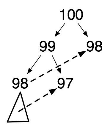
The problem is that there is overlap in the computations done by the two recursive applications. The computation of (fib 100) recursively applies (fib 98) twice, and (fib 97) three times. There is even more repetition of applications with smaller arguments (not shown in the diagram).
We can eliminate the repeated computations by maintaining a list of already-computed pairs \((n, F_n)\).
| (define fib-table empty) |
| (define (memo-fib n) |
| (define result (assoc n fib-table)) |
| (cond |
| [result => second] |
| [else |
| (define fib-n |
| (cond |
| [(= n 0) 0] |
| [(= n 1) 1] |
| [else (+ (memo-fib (- n 1)) |
| (memo-fib (- n 2)))])) |
| (set! fib-table (cons (list n fib-n) fib-table)) |
| fib-n])) |
Note the use of the built-in function assoc, which works on association lists such as the one we have constructed, and two additional features of full Racket: any non-false value (not just true) for a cond question causes the associated answer to be evaluated, and the => causes that value to be provided as the argument to the function produced by evaluating the answer. We would have had to write [(list? result) (second result)] in the teaching languages.
This reduces the "tree of computations" started in the above diagram to just the computations down the left spine. Right children are looked up in the association list and there is no branching of the tree beneath them.
In this program, fib-table is a global variable, but there is no need for it to be exposed to any code other than memo-fib. We can limit its scope in the following fashion.
| (define memo-fib |
| (local |
| [(define fib-table empty) |
| (define (memo-fib n) ...)] |
| memo-fib)) |
This technique will not quite work for the address-book example we saw earlier, because in that example, the global variable address-book needed to be in scope for two functions, add and lookup. The Racket form define-values can be used in a similar fashion for that example.
We have seen a use of set! for improving efficiency. It can also be used to improve expressivity in certain cases. If the body of function f applies function g, and function g needs a value that f can compute, then that can be passed down as an additional parameter to g. But if f does not directly apply g (for example, it applies h, which applies g, or maybe the chain is even longer), then the additional parameter has to be added to every intermediate function. This can get messy and awkward if it has to be done often.
We could, instead, define a variable in the scope of both f and g, and have f mutate it to the computed value. This also works in the case where f and g are both applied during a computation, but there is no direct path between them in the computation tree.
A number of bindings for values that affect the operation of a Racket program are treated in this fashion, using a Racket feature that is also confusingly known as parameters. For example, there is a parameter for the current default output port, the one that display uses when no port argument is given. This parameter is current-output-port. A program can query its value using (current-output-port), but can also set its value with an expression like (current-output-port my-port).
A common pattern for using parameters is to set them temporarily, and then reset them once a computation is done. The parameterize form does this. In effect, this use of parameters is a form of dynamic scope.
| (parameterize ([current-output-port my-port]) |
| (my-function-that-does-output)) |
You can now see how functions like with-output-to-file can be written in just a few lines. The function make-parameter allows the programmer to create their own parameters. While this may seem a lot of work for what looks like something that can easily be done with set! expressions, parameters work properly with non-standard control flow such as can happen with threads and continuations. I will discuss these in later chapters. In the meantime, be aware that there are two meanings for the word "parameter", though I usually intend the meaning familiar from Part I.
2.10 Intermediate mutation
The limitations of elementary mutation become apparent when we try to generalize the address book example to maintain an arbitrary number of address books. We want one "add" function for all address books, so it is natural to try to make the address book be a function parameter. Here is an attempt which fails.
| (define work '(("Arturo Belano" 6345789) |
| ("Ulises Lima" 2345789))) |
| (define home '()) |
| (define (add-entry abook name number) |
| (set! abook (cons (list name number) abook))) |
| (add-entry home "Maria Font" 2076543) |
| home |
We might expect the last expression to evaluate to '(("Maria Font" 2076543)), but instead it evaluates to '(). We have three problems to solve: the code does not work, it is not clear how to get it to work, and we cannot explain (using the substitution model) what the code actually does.
It is not even clear how to do the substitution into the body of add-entry when evaluating (add-entry home "Maria Font" 2076543). We need to substitute '() for abook in (set! abook (cons (list name number) abook)). Substituting for the second occurrence makes sense, but not the first one. Even if we leave the first occurrence alone, the resulting set! expression will be grammatically correct, but the reduction rule for the substitution model cannot be applied, as there is no (define abook ...) statement.
Intuitively, the code is mutating a local copy of the address book argument, and not the global variable. To model what the incorrect code is actually doing, we would need to perform the rewrite as follows.
| (add-entry home "Maria Font" 2076543) |
| => (add-entry '() "Maria Font" 2076543) |
| => (local |
| [(define abook '()) |
| (define name "Maria Font") |
| (define number 2076543)] |
| (set! abook (cons (list name number) abook))) |
Since the code does not work anyway, and in general mutation of function parameters is of little use in Racket, I will not pursue this line of thought. Instead, I’ll focus on creating code for multiple address books that actually works.
To do this, I’ll go back to our simulation of structures using lambda, at the beginning of section 6.7 in Part I, and use it to simulate boxes. A box can be thought of as a struct with one field that supports two operations, "getting" the value of the field, and "setting" it to a new value (mutation). Boxes are a standard feature in Racket, but if we build them ourselves first (as we did with lists), we will understand how they work.
Here is the version without mutation, based on the code from Part I.
| (define (make-box v) |
| (lambda (msg) |
| (cond |
| [(equal? msg 'get) v]))) |
| (define (get b) (b 'get)) |
In Part I, we needed the cond because the structure we were simulating had two fields, so the lambda accepted two different messages. We only have one message so far, but we will add a 'set message shortly. Let’s trace an example of the use of the code we have right now.
| (define b1 (make-box 7)) |
| (get b1) |
| => |
| (define b1 |
| (lambda (msg) |
| (cond |
| [(equal? msg 'get) 7]))) |
| (get b1) |
| => |
| (get (lambda (msg) |
| (cond |
| [(equal? msg 'get) 7]))) |
| => |
| ((lambda (msg) |
| (cond |
| [(equal? msg 'get) 7])) 'get) |
| => |
| (cond [(equal? 'get 'get) 7]) |
| =>* 7 |
In Racket, the functionality we have put into make-box is provided by box, and the equivalent of our get is unbox.
We need a definition in order to use elementary mutation (set!), so we change the code to put the value into a local variable.
| (define (make-box v) |
| (local [(define val v)] |
| (lambda (msg) |
| (cond |
| [(equal? msg 'get) val])))) |
| (define (get b) (b 'get)) |
To be sure we haven’t broken anything, let’s repeat our trace on the same example.
| (define b1 (make-box 7)) |
| (get b1) |
| => |
| (define b1 |
| (local [(define val 7)] |
| (lambda (msg) |
| (cond |
| [(equal? msg 'get) val])))) |
| (get b1) |
| => |
| (define val_1 7) |
| (define b1 |
| (lambda (msg) |
| (cond |
| [(equal? msg 'get) val_1]))) |
| (get b1) |
| => |
| (define val_1 7) |
| (get (lambda (msg) |
| (cond |
| [(equal? msg 'get) val_1]))) |
| => |
| (define val_1 7) |
| ((lambda (msg) |
| (cond |
| [(equal? msg 'get) val_1])) 'get) |
| => |
| (define val_1 7) |
| (cond [(equal? 'get 'get) val_1]) |
| =>* 7 |
Now we can add the 'set message. But setting requires additional information, namely the new value. One way to handle this is to have the response to the 'set message be another lambda that consumes the new value and does the mutation.
| (define (make-box v) |
| (local [(define val v)] |
| (lambda (msg) |
| (cond |
| [(equal? msg 'get) val] |
| [(equal? msg 'set) |
| (lambda (newv) |
| (set! val newv))])))) |
| (define (get b) (b 'get)) |
| (define (set b v) ((b 'set) v)) |
The Racket equivalent to our set is set-box! Let’s trace an example of a use of set.
| (define b1 (make-box 7)) |
| (set b1 4) |
| => |
| (define b1 |
| (local [(define val 7)] |
| (lambda (msg) |
| (cond |
| [(equal? msg 'get) val] |
| [(equal? msg 'set) |
| (lambda (newv) |
| (set! val newv))])))) |
| (set b1 4) |
| => |
| (define val_1 7) |
| (define b1 |
| (lambda (msg) |
| (cond |
| [(equal? msg 'get) val_1] |
| [(equal? msg 'set) |
| (lambda (newv) |
| (set! val_1 newv))]))) |
| (set b1 4) |
| => |
| (define val_1 7) |
| (define b1 |
| (lambda (msg) |
| (cond |
| [(equal? msg 'get) val_1] |
| [(equal? msg 'set) |
| (lambda (newv) |
| (set! val_1 newv))]))) |
| ((b1 'set) 4) |
| =>* |
| (define val_1 7) |
| ((lambda (newv) (set! val_1 newv)) 4) |
| => |
| (define val_1 7) |
| (set! val_1 4) |
| => |
| (define val_1 4) |
At this point it is clear that evaluating (get b1) would produce 4 and not the initial value 7 that was stored in the box.
The point of our homebrewed implementation of boxes is to motivate the additions to the substitution model necessary to explain the boxes that Racket provides. We will create substitution rules for expressions involving boxes that mimic what happens in our simulation.
Here are the grammatical rules for boxes. Notice that the first parameter of set-box! is an expression (that produces a box value) instead of an identifier as was the case with the first parameter of set!.
| exp | = | (box exp) | ||
| | | (unbox id) | |||
| | | (set-box! exp exp) |
Before I explain the reduction rules, let’s look at how to use boxes to solve the problem of multiple address books.
| (define home (box '((Mom 8884567) |
| (Sis 7001234)))) |
| (define work (box '((Boss 39751)))) |
| (define (add-entry abook name phone) |
| (set-box! abook |
| (cons (list name phone) |
| (unbox abook)))) |
| (add-entry work 'Intern 666) |
Our rewrite rules for the built-in box functions will use the same idea as our simulation. This suggests that the semantics of box should create a define expression. set-box! can then act on the created definition in the same manner as set! does for names.
The semantic rule for rewriting (box v) (where v is a value) will be to introduce a new top-level expression (define u v) where u is a new, unique name not used elsewhere. This new name will also be considered a Scheme value.
The (box v) expression is replaced by this name, but here and anywhere the new name appears in an expression, it is not rewritten.
The semantic rule for rewriting (unbox n) (where n is one of these new, unique names that is a value) is to find a (define n v) expression, and replace (unbox n) by v.
Finally, the semantic rule for rewriting (set-box! n v) is to find the define expression involving n, rewrite it so that it is (define n v), and replace the (set-box! n v) expression with (void).
Let’s trace an example with the new rules.
(define box1 (box 4)) ; to be rewritten next (unbox box1) (set-box! box1 true) (unbox box1) => (define box1 unique_1) (define unique_1 4) (unbox box1) ; to be rewritten next (set-box! box1 true) (unbox box1) => (define box1 unique_1) (define unique_1 4) 4 (set-box! box1 true) ; to be rewritten next (unbox box1) => (define box1 unique_1) (define unique_1 true) 4 (unbox box1) ; to be rewritten next => (define box1 unique_1) (define unique_1 true) 4 true
The two definitions represent the mapping from the name box1 to the location where the box’s value is stored, and the mapping from the location (the definition of unique_1) to the value contained in the box (true).
These reduction rules are less intuitive than previous reduction rules, and this is one of the problems with mutation. The substitution model, which was of considerable use in understanding recursive functions, becomes less useful when mutation is involved. The memory model introduced more fully in the next chapter helps us cope with this.
2.11 Advanced mutation
Advanced-level mutation features in Racket include mutable structures and lists. There are no structures in R5RS (standard) Scheme, and in that language, cons fields are mutable with set-car! and set-cdr!.
In Racket, cons fields are immutable, and this is a major departure from longtime standard practice in Scheme and Lisp. The reasons for this are explained in this Racket blog post.
Racket does provide a separate datatype for mutable pairs: mcons is mutable with mset-car! and mset-cdr!. As for structures, struct and define-struct accept the keyword #:mutable, which indicates that the fields of the given structure are mutable.
| (struct posn (x y) #:mutable) |
| (define p (posn 3 4)) |
| (set-posn-x! p 5) |
| (posn-x p) => 5 |
We can generalize the semantic rules for boxes to apply to structures. In the semantics of structures discussed in Part I, a make-posn expression was considered a value and not rewritten. But this cannot be the case for mutable structures. Just as the box function created a definition to hold the value, the make-posn should create a definition. But that definition has to hold two values, because a posn structure has two fields. We will use a make-posn* expression in the definition, the asterisk * indicating that the expression is not to be rewritten.
| (define p1 (make-posn 3 4)) |
| => |
| (define unique_1 (make-posn* 3 4)) |
| (define p1 unique_1) |
Here, as before, the new, unique name in the definition is considered a value and not rewritten.
The semantics of (posn-x n), where n is one of these new, unique names, is to replace the expression by the first value stored in the make-posn* expression appearing in the definition of n.
| (define p1 (make-posn 3 4)) |
| (posn-x p1) |
| => |
| (define unique_1 (make-posn* 3 4)) |
| (define p1 unique_1) |
| (posn-x p1) |
| => |
| (define unique_1 (make-posn* 3 4)) |
| (define p1 unique_1) |
| (posn-x unique_1) |
| => |
| (define unique_1 (make-posn* 3 4)) |
| (define p1 unique_1) |
| 3 |
The semantics of (set-posn-x! n v) is to replace by v the first value appearing in the make-posn* expression in the definition of n.
| (define p1 (make-posn 3 4)) |
| (set-posn-x! p1 5) |
| => |
| (define unique_1 (make-posn* 3 4)) |
| (define p1 unique_1) |
| (set-posn-x! p1 5) |
| => |
| (define unique_1 (make-posn* 3 4)) |
| (define p1 unique_1) |
| (set-posn-x! unique_1 5) |
| => |
| (define unique_1 (make-posn* 5 4)) |
| (void) |
We can generalize this to a structure with any number of fields, and to mutable mcons cells.
As you can see, the rules work, they are not very complicated (less so than the rule for local), and there aren’t many of them. However, tracing mutation-heavy code by hand or with a Stepper using these rules is not very illuminating. It will provide us with the right answer, but not with the intuition needed to write such code properly. The memory model, as presented later, does not provide complete semantics, but gives a better intuitive understanding of the effects of mutation. The semantics in the memory model can be completed to handle all the Racket language features we know about, but the result (especially for function application, recursion, and the treatment of functions as values) is much more complicated than the substitution model.
The presence of boxes or mutable structures exposes details that require a shift in our thinking. Consider the following example.
| (define lst1 (cons (box 1) empty)) |
| (define lst2 (cons 2 lst1)) |
| (define lst3 (cons 3 lst1)) |
| (set-box! (first (rest lst2)) 4) |
| (unbox (first (rest lst3))) |
| => ? |
Thinking as we did in Part I, we would think of lst2 as the value (list 2 (box 1)) and lst3 as the value (list 3 (box 1)). But in fact the two boxes are the same, as we could see if we trace this code using the semantics we discussed in the previous lecture module. So when we change the value in the box in lst2, and then look at the box in lst3, it contains the new (mutated) value. This kind of sharing is not visible without mutation. It is a source of added complications, which the memory model can help us manage.
In the rewriting semantics associated with mutation, we see the phenomenon that a single step rewriting an expression may involve finding and modifying a definition elsewhere in the program.
| (define x 3) (set! x 7) x |
| => (define x 7) (void) x |
| => (define x 7) x |
| => (define x 7) 7 |
I wrote before of a definition being a name-value binding. But now we see a more subtle way of viewing that relationship. A name-value binding is a name-location mapping (the location being where the define is) plus a location-value mapping (given by the contents of the define).
The form set! changes the location-value mapping (by rewriting the define). But it does not change the name-location mapping. Something similar happens with the other forms of mutation.
| (define x (box 3)) |
| (set-box! x 7) |
| => |
| (define x uniquev) |
| (define uniquev 3) |
| (set-box! x 7) |
| => |
| (define x uniquev) |
| (define uniquev 3) |
| (set-box! uniquev 7) |
| => |
| (define x uniquev) |
| (define uniquev 7) |
| (void) |
And it even happens with local.
| (local [(define x 7)] x) |
| => |
| (define x_unique 7) |
| ... |
| x_unique |
Each of these features treat a define as a place where information can be stored. This idea is important to keep in mind as we proceed.
2.12 Adding mutation to an interpreter
In the Interpreters chapter of Part I, we looked at three kinds of interpreters: small-step (following the rewrite rules of our computational model for Racket), big-step (evaluation) with explicit substitution, and big-step with deferred substitution using environments. Here we will focus on adding mutation to the environment-passing interpreter. You may wish to review section 10.6 of Part I in preparation. Starter code for the interpreter from Part I, but using the new features of full Racket introduced above, is linked in the Handouts chapter.
We implemented an environment as an association list of name-value bindings representing deferred substitutions. The trickiest part was the evaluation of lambda expressions; this creates a closure, a value that includes the syntactic information from the lambda (parameter name and body expression) as well as the environment at the time of creation. That environment is used when the lambda is applied; it is extended with a new binding of the parameter name to the argument value, after which the body of the lambda is interpreted in the extended environment.
Some kinds of expressions do not require environment extensions, and the current environment is used to recursively evaluate subexpressions. This would be the case for the evaluation of '(+ exp1 exp2); both exp1 and exp2 are recursively evaluated in the current environment. Taking advantage of match, and postulating a plus AST structure, the code would look something like this:
| (define (interp exp env) |
| (match exp |
| ... |
| [(plus exp1 exp2) (+ (interp exp1 env) |
| (interp exp2 env))] |
| ...)) |
For new language features, we add to the grammar and to the set of AST structures. Previously, in Faux Racket, I used the same surface syntax as Racket, but now I’ll change it. I’ll use set for mutation in Faux Racket (set! in Racket) and seq for sequencing in Faux Racket (begin in Racket).
| exp | = | (set id exp) | ||
| | | (seq exp exp) |
The obvious thing to try, in implementing mutation, is to evaluate the body subexpression in the set, and then to add to the environment a binding of id to the resulting value (perhaps removing any existing binding of id). This is incorrect, and it’s important to understand why.
Consider the following Faux Racket code:
| (with ((x 0)) |
| (+ (seq (set x 5) x) |
| (seq (set x 6) x))) |
This should evaluate to 11. If we change the binding of x during evaluation of the first argument of +, we must then use the changed environment to evaluate the second argument. But this risks violating the scope rules in the absence of mutation. If the first argument to + is a let subexpression, the extended environment from that shouldn’t be used to evaluate the second argument of + (the scope of the binding created by let is just its body expression). Then again, if the let subexpression contains a mutation of a variable whose scope includes both arguments of +, we do want that to persist when the second argument is evaluated. Trying to figure out the rules seems difficult.
The solution to the dilemma is to apply the reasoning at the end of the previous section, where a name-value binding was considered as a combination of a name-location binding and a location-value binding. The environment will manage name-location bindings, and the management of environments will not change in our interpreter. Location-value bindings will be kept in a separate association list we will call the store, which will be threaded through the computation (by making it both an additional parameter to the interpreter and part of what the interpreter produces) to give the dynamic effect of mutation. A location can be any value that can be tested for equality; we can, for example, use natural numbers for locations.
Here’s what the code for the case I used as an example just above might look like with the store integrated.
| (struct result (val store)) |
| (define (interp exp env sto) |
| (match exp |
| ... |
| [(plus exp1 exp2) |
| (define res1 (interp exp1 env sto)) |
| (define res2 (interp exp2 env (result-store res1))) |
| (result (+ (result-val res1) (result-val res2)) |
| (result-store res2)) |
| ...])) |
What else has to change in the old interpreter? Looking up a variable now is a two-step process: use the name to look up the location in the environment, and then use the location to look up the value in the store. For function application, in addition to threading the store through the two recursive applications of the interpreter (for the expression in "function" position and the expression in "argument" position), we must create a new location to hold the value of the argument, and add a name-location binding to the environment. The easiest way to create a new location (natural number) is to use the length of the association list holding the store.
Adding code for the seq case is similar to what we see above. For "set", we evaluate the body expression, use the name of the variable being mutated to look up its location, then add a new location-value binding to the store (optionally removing the old binding, as it will never be used again).
The fact that we never remove a location from the store makes a long computation with this interpreter impractical. A more practical interpreter would remove or reuse unused locations (such as the one used for the argument of an applied function, which is unused after the result is computed). This process is called garbage collection, and is a standard feature of modern programming languages. I’ll talk about this in a later chapter.
The semantics of function application in this interpreter explains the behaviour of our bad implementation of the address book in the section on elementary mutation. The use of set! in the incorrect code mutates only a local copy of the argument. We can change the rewriting model for Racket to treat function application in this fashion, but it further renders the model impractical. It is easier to avoid mutating parameters, since this has very little use in typical Racket code.
Exercise 3: Complete the implementation of the store-passing interpreter. \(\blacksquare\)
Exercise 4: The designers of Scheme made relatively few mistakes, but arguably one of them was to include set! instead of boxes. Remove the implementation of set! from your answer to the previous exercise, and instead implement box, unbox, and set-box!. \(\blacksquare\)
Exercise 5: The letrec construct in standard Scheme is also available in Racket. It resembles local, but its syntax is closer to let. In this question, you will add rec (implementing letrec) and ifzero (implementing zero?) to the old interpreter from Part I without mutation. Just as that interpreter implemented a version of let permitting just one binding, rec is a version of letrec permitting just one binding. Here is the grammar for the interpreted language.
| expr | = | num | ||
| | | var | |||
| | | (+ expr expr) | |||
| | | (* expr expr) | |||
| | | (- expr expr) | |||
| | | (/ expr expr) | |||
| | | (fun (var expr)) | |||
| | | (ifzero expr expr expr) | |||
| | | (let ((var expr)) expr) | |||
| | | (rec ((var expr)) expr) |
Why is the implementation of rec harder than let? Consider interpreting an expression of the form (rec ((x E)) B), where E and B are arbitrary expressions. We need to interpret E in the current environment e, which does not have a binding for x, even though x may be mentioned in E. If x is mentioned in E, it should be in the body of a fun, and those are not interpreted until the function is applied, so the binding of x will not be needed during the interpretation of E. However, if E evaluates to a closure c, then c contains an environment f, and f will extend e and thus not have a binding for x. So c cannot be bound to x and successfully used to evaluate B (unless B does not mention x at all).
We can create a closure d whose environment g extends f with a binding for x (and can thus be successfully used to evaluate B), but what should that binding be? It should be to d. The data structure is circular, and circular data structures cannot be created using pure code.
One efficient solution to this problem is to use a mutable structure for closures by adding the keyword #:mutable. We can then create d with a "dummy" value in the environment field (say, the value 'undefined), create the extended environment g, and then mutate the environment field of d so that its new value is g. This is the only use of mutation you will need in your interpreter. \(\blacksquare\)
2.13 Memory and vectors

(Salvador Dali, The Persistence of Memory, 1931. Now in the collection of the Museum of Modern Art, New York City.)
Computers, such as the ones that run Racket programs, have specific methods of storing and retrieving information that become relevant in working with mutation, and in working with languages such as C where mutation is central instead of peripheral. In discussing these methods, I will abstract away some of the details, and some of the differences among different types of computers, but will remain reasonably faithful to reality. The subject is treated more carefully in textbooks on computer architecture, and at considerable length in the field of Computer Engineering.
Memory in a modern computer resembles a set of numbered mailboxes. The numbers are called addresses.
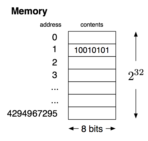
Each box can store only eight bits (a "byte"), though they are often grouped into sets of four (a "word" in a 32-bit architecture) or eight (in a 64-bit architecture). The number of boxes depends on the machine, but usually does not exceed \(2^{32}\) (the number of different addresses that can be specified with 32 bits) for a 32-bit architecture, and \(2^{64}\) (effectively no practical bound) for a 64-bit architecture.
The dominant data structure in many early computer languages (and this is still true for the C programming language, originally designed in the 1970’s) was the array, which is a thin abstraction for a sequence of consecutive memory locations. Arrays are like "living fossils" such as sharks, in that they are a modern manifestation of something that stopped evolving some time ago.
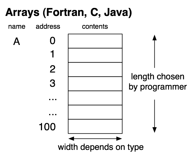
Each element of an array in such languages is of a fixed size (say, a 32-bit integer). The IYMLC flânerie goes into more detail on C arrays. Here we will look at a similar datatype in Racket (and standard Scheme). This is the vector, addressed in a manner similar to C. The difference is that a Scheme or Racket vector can, like lists, contain unbounded values, and values of different types.
Exercise 6: An exercise in Part I asked you to implement an ADT for natural numbers while pretending that Racket did not support numbers. The exercise used "slists", or lists of symbols, to represent numbers. In this question, you will implement the ADT again, but under the assumption that Racket integers have the same restrictions as C integers (that is, the legal range is \(-2,147,483,648\) to \(2,147,483,647\)). You should never produce a numeric value outside this range. (This restriction is a consequence of using exactly 32 bits to represent an integer.)
Since we can use numbers of moderate size, our representation of unbounded numbers will be as lists of "big digits", where a big digit, or bigit, is from \(0\) to \(9999\). (In effect, we are representing a large number in base \(10000\). The reason for this choice is that multiplying two bigits will not result in overflow, and that "reading" this representation is pretty easy for humans.)
More precisely, the blist (short for "bigit list") representing \(n\) is empty if \(n=0\), or if \(n>0\) it is (cons b bl), where b is a bigit, bl is a blist representing \(k\), and \(n=10000k+b\).
In a fashion similar to the exercise in Part I, write the utility functions nat-to-blist and blist-to-nat to help in your testing (here you can violate the restrictions on Racket integers, of course). You should use these only for testing, and not to implement the next two functions, which are add and mult. These consume and produce blists, with the same efficiency considerations as in the Part I exercise. Do not use mutation. (This should be a straightforward generalization of the earlier exercise, and is a useful intermediate step for a similar exercise in IYMLC.) \(\blacksquare\)
2.14 Vectors in Racket
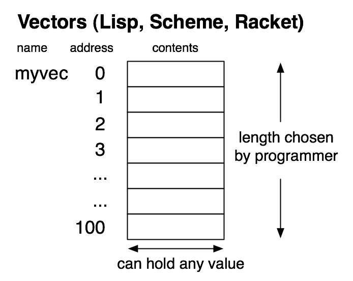
A vector may be created in Racket with the built-in function vector, which makes a vector from the sequence of arguments.
(define x (vector 'blue true "you"))
We can make longer vectors with make-vector, which consumes a length (and optional initial value for each element), and with build-vector, which is similar to build-list.
| (define y (make-vector 100)) |
| (define z (build-vector 100 sqr)) |
We extract the value of an element by providing vector-ref with two arguments, a vector and an index (a natural number). We can modify the value of an element by providing vector-set! with these two arguments plus a third, the new value.
| (define y (make-vector 100 5)) |
| (vector-ref y 7) => 5 |
| (vector-set! y 7 42) |
| (vector-ref y 7) => 42 |
The big advantage of a vector is that (due to the similarity with actual memory in the machine) vector-ref and vector-set! each have constant running time. Set against this considerable advantage are some disadvantages. Vectors have a fixed size. One cannot add additional elements to them easily, or remove elements. Using vector-set!, as with other mutation constructs, tends to require a different style of programming, harder to reason about and get correct.
Creating our own implementation of build-vector gives us some experience in working with vectors.
| (define (my-build-vector n f) |
| (define res (make-vector n)) |
| (define (mbv-h i) |
| (cond |
| [(= i n) res] |
| [else |
| (vector-set! res i (f i)) |
| (mbv-h (add1 i))])) |
| (mbv-h 0)) |
We are seeing a common pattern in these small functions, and it is not surprising that Racket provides a number of iteration constructs (implemented using macros) to facilitate writing them. Here are two more implementations, with the same functionality as the one above, but using Racket’s for and for/vector constructs, respectively. You can read more about these in the "Iterations and Comprehensions" section of the Racket Guide and the Racket Reference.
| (define (my-build-vector2 n f) |
| (define res (make-vector n)) |
| (for ([i n]) |
| (vector-set! res i (f i))) |
| res) |
| (define (my-build-vector3 n f) |
| (for/vector ([i n]) (f i))) |
Here is another example, a function that adds up a vector of numbers. Note the manner, similar to quote notation, in which a vector value can be specified; this is also the way that vectors are printed.
| (define (sum-vector vec) |
| (define (sv-h i acc) |
| (cond |
| [(= i (vector-length vec)) acc] |
| [else |
| (sv-h (add1 i) |
| (+ acc |
| (vector-ref vec i)))])) |
| (sv-h 0 0)) |
| (sum-vector #(1 2 3 4 5)) => 15 |
We could take the accumulator out and make it a local variable that is manipulated through mutation. This really offers no advantages at all in Racket. Please do not program in Racket in this manner; it is being done here for purposes of illustration. The implementation below has very similar time and space efficiency as the one above.
| (define (sum-vector2 vec) |
| (define acc 0) |
| (define (sv-h i) |
| (cond |
| [(= i (vector-length vec)) acc] |
| [else |
| (set! acc |
| (+ acc |
| (vector-ref vec i))) |
| (sv-h (add1 i))])) |
| (sv-h 0)) |
We can go further along these lines and pull out the other parameter as well. This is considered bad form in Racket (and Scheme), and once again, do not program like this in Racket. This program resembles the way programs are written in C and other imperative languages that are more rooted in the past and offer inadequate support for functions. We will soon take some of the ideas of programs like this and use them to design our own small, artificial, imperative language (in the next chapter).
| (define (sum-vector3 vec) |
| (define acc 0) |
| (define i 0) |
| (define (sv-h) |
| (cond |
| [(= i (vector-length vec)) acc] |
| [else |
| (set! acc |
| (+ acc |
| (vector-ref vec i))) |
| (set! i (add1 i)) |
| (sv-h)])) |
| (sv-h)) |
It is worth examining the helper function sv-h in this code more carefully. It produces a value, but that value is just the value of the externally-defined variable acc; we could easily have written it to produce the useless value #<void>, and accessed the value of acc as the last expression in the body of sum-vector3.
| (define (sum-vector4 vec) |
| (define acc 0) |
| (define i 0) |
| (define (sv-h) |
| (cond |
| [(= i (vector-length vec)) (void)] |
| [else |
| (set! acc |
| (+ acc |
| (vector-ref vec i))) |
| (set! i (add1 i)) |
| (sv-h)])) |
| (sv-h) |
| acc) |
Furthermore, sv-h has no parameters; it uses tail recursion, and only does so in order to repeat a computation that is entirely concerned with manipulating state. It makes little or no sense to program this way in Racket; we have much better ways of achieving the same goals.
We can use Racket’s iteration constructs to simplify the code for this task. Below is another use of for, followed by another solution that uses the for/fold construct.
| (define (sum-vector5 vec) |
| (define sum 0) |
| (for [(i (vector-length vec))] |
| (set! sum |
| (+ sum (vector-ref vec i)))) |
| sum) |
| (define (sum-vector6 vec) |
| (for/fold [(sum 0)] |
| [(v (in-vector vec))] |
| (+ sum v))) |
Which of the previous implementations is sum-vector6 an abstraction of? It doesn’t really matter. We can consider it purely functional even if the implementation involves mutation, because that is hidden from us. This is another way to tame the problems caused by mutation: hide it behind a purely functional interface.
Given that memory is in fact made up of fixed-size slots which cannot store arbitrary values, it is reasonable to ask what a Racket vector actually is. It is implemented as a C-style vector of fixed-length descriptions (memory addresses) where the real values can be found. Those values may take up an arbitrary number of memory locations (for example, if they are very large integers).
Each cons is a pair of such fixed-length descriptions. We often use a graphical notation known as "box-and-pointer diagrams" to aid in understanding such data structures. The pointers are an abstraction of memory addresses.
(cons 'blue (cons true empty))
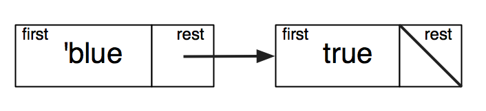
(cons 1 (cons 'blue (cons true empty)))
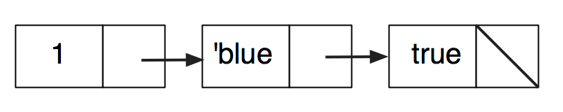
Though we tend to use diagrams like the ones above, the one below is perhaps more accurate with respect to the actual implementation:
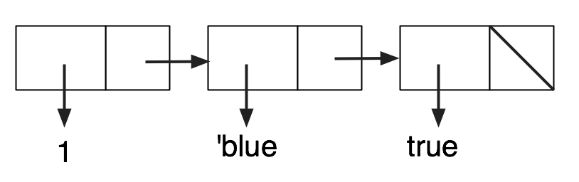
Even this may not be fully accurate, because the implementation of Racket uses various optimizations to minimize the number of pointers where possible. But it’s a better view to keep in mind.
The treatment of structures generalizes that of cons. Each struct consists of as many such fixed-length descriptions (addresses) as there are fields.
Because Racket is dynamically typed, each value in memory must include type information. I have not included this in the above pictures, and will go into more detail later.
For a nontrivial application of vectors (and one that is very important in practice), I’ll discuss a data structure that is better in practice than association lists (even though its worst-case running time is no better). However, this implementation will have some significant differences from the implementations we saw in Part I. We will need a modified conceptual framework to deal with this.
2.15 Abstract data types with state
In Part I, I gave a mathematical definition of sequences, in order to introduce the list data structure. Later, because I wanted to give an alternate representation using binary trees, I was more careful about defining operations on sequences. Those definitions together constitute an abstract data type (ADT), which is a mathematical description of a data type and a set of operations on it.
Here I’ll review that definition and be even more precise. Each operation will have a set of parameters, a precondition describing when the operation can be applied to a given set of arguments, and a postcondition describing the value produced. The precondition can be true if the operation can always be applied.
This is the definition of what I’ll call the Sequence ADT, taken from Part I.
A sequence \(S\) of \(k\) elements is usually represented in mathematics as \(S = s_0, s_1, \ldots, s_k\); the length of this sequence is \(k+1\). Here are the operations of the immutable Sequence ADT.
empty: no parameters; precondition true; value produced is the empty sequence.
add: two parameters, an element \(e\), and a sequence \(S = s_0, s_1, \ldots, s_k\); precondition true; value produced is \(S' = e, s_0, s_1, \ldots, s_k\).
first: one parameter, a sequence \(S = s_0, s_1, \ldots, s_k\); precondition \(\mathit{length}~S>0\); value produced is \(s_0\).
remove: one parameter, a sequence \(S = s_0, s_1, \ldots, s_k\); precondition \(\mathit{length}~S>0\); value produced is \(S = s_1, \ldots, s_k\).
index: two parameters, a natural number \(i\) and a sequence \(S = s_0, s_1, \ldots, s_k\); precondition \(\mathit{length}~S > i\); value produced is \(s_i\).
This ADT is immutable. Operations produce a new value and do not modify existing values. ADT definitions are used a lot in computer science, and they tend to be slightly different when state is involved. With mutable ADTs, the values of the defined type are each conceptually contained in a state variable. For the ADT definition, we think of one state variable per value, though an implementation may use several variables to represent that value. A postcondition for a mutable ADT includes description of side effects (typically on that state variable, but may also involve I/O). An operation may now be performed only for side effects and not produce a value.
For the mutable Sequence ADT, the first and index operations are the same. The empty operation creates a new sequence whose state variable is the empty sequence. The add and remove operations are changed.
add: two parameters, an element \(e\), and a sequence \(S = s_0, s_1, \ldots, s_k\); precondition true; no value produced; postcondition is that \(S\) has value \(e, s_0, s_1, \ldots, s_k\).
remove: one parameter, a sequence \(S = s_0, s_1, \ldots, s_k\); precondition \(\mathit{length}~S>0\); no value produced; postcondition is that \(S\) has value \(s_1, \ldots, s_k\).
We can create a flawed implementation of the mutable Sequence ADT using a mutable structure with two fields, one holding a vector and one holding a natural number that is an index into the vector one greater than where the first element of the sequence is stored.
| (struct seq (vec idx) #:mutable) |
| (define (make-empty) (seq (make-vector LENGTH) 0)) |
| (define (first s) (vector-ref (seq-vec s) (sub1 (seq-idx s)))) |
| (define (add e s) |
| (define i (seq-idx s)) |
| (vector-set! (seq-vec s) i e) |
| (set-seq-idx! s (add1 i))) |
| (define (remove s) |
| (set-seq-idx! s (sub1 (seq-idx s)))) |
The flaw in this implementation, and it is a big one, is that the length of the vector has to be a fixed constant LENGTH chosen before any operations are performed. If we choose this too small, it will not be able to hold all elements of the sequence, and if we choose it too large, we will waste space. But if we can live with this limitation, and all the other drawbacks of working with mutation this implements all operations in constant time, which is better than the implementations for the immutable ADT (Braun trees achieved logarithmic time).
This data structure, though simple, is useful enough that it has a name: a stack. The add operation is usually called push, and the remove operation is usually called pop. We will see that this data structure plays a critical role in the implementation of programming languages.
The ADT that association lists implement is usually called Map, Table, or Dictionary. Here is an immutable Map ADT.
A map is a set of (key,value) pairs.
make-map: no parameters; precondition true; value produced is \(M\), with postcondition \(M = \phi\).
add: three parameters, a map \(M\), a key \(k\), and a value \(v\); precondition true.
The value produced is \(M'\), with postcondition that if there exists a value \(v'\) such that \((k,v')\in M\), then \(M' = M \setminus \{(k,v')\} \cup \{(k,v)\}\), otherwise \(M' = M \cup \{(k,v)\}\).
remove: two parameters, a map \(M\) and a key \(k\); precondition true;
The value produced is \(M'\) with postcondition that if there exists a value \(v\) such that \((k,v)\in M\), then \(M' = M \setminus \{(k,v)\}\), otherwise \(M' = M\).
search: two parameters, a map \(M\) and a key \(k\); precondition true; value produced is \(v\) such that \((k,v)\in M\), otherwise something not in value domain.
Now I’ll define the mutable Map ADT.
make-map and search are the same as in the immutable Map ADT.
add: three parameters, a map \(M\), a key \(k\),
and a value
\(v\); precondition true; produces no value; postcondition is that if
there exists a value \(v'\) such that \((k,v')\in M\), then \(M \leftarrow M
\setminus \{(k,v')\} \cup \{(k,v)\}\), otherwise \(M \leftarrow M \cup \{(k,v)\}\).
The \(\leftarrow\) notation makes the mutation of the state variable \(M\) explicit.
remove: two parameters, a map \(M\) and a key \(k\); precondition true; produces no value; postcondition is that if there exists a value \(v\) such that \((k,v)\in M\), then \(M \leftarrow M \setminus \{(k,v)\}\), otherwise \(M\) is unchanged.
Next, I’ll discuss the implementation of the mutable Map ADT. For simplicity, I assume that the keys are integers, and omit the associated values from diagrams. Since every key appears at most once, ignoring the values means that we are representing sets, though the operations are different than the ones we defined when we talked about sets in Part I.
The problem with using an association list to implement the Map ADT is that there is only one list, and access to the last element of the list takes time proportional to the number of elements. This means that searches for that last element (or unsuccessful searches) take a long time. The elements of vectors, on the other hand, can be accessed in constant time. If we create a vector whose size is the maximum value of a key, and store the value associated with key \(k\) at index \(k\), then a search can be done in constant time. But this will waste space unless the maximum value of a key is guaranteed to be a small number (and keys cannot be negative).
One possible solution is to combine the two ideas, by using a vector of several association lists. This is one variant of what is known as a hash table.
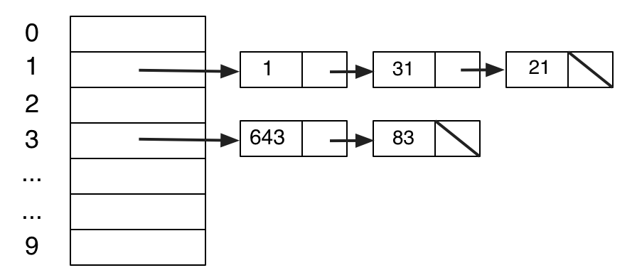
(define (create-hashtable size) (make-vector size empty))
To see which association list to use for a (key,value) pair, we map the key into the range of vector indices. This mapping is called a hash function. For simplicity, here I’ll use remainder on division by the vector length. Depending on the data, that may not distribute keys evenly, so typically a more complicated hash function is used.
| (define (ht-search table key) |
| (define index (modulo key |
| (vector-length table))) |
| (define hashlist (vector-ref table index)) |
| (define lookup (assoc key hashlist)) |
| (if lookup (second lookup) false)) |
| (define (ht-add table key val) |
| (define index (modulo key (vector-length table))) |
| (define hashlist (vector-ref table index)) |
| (define lookup (assoc key hashlist)) |
| (if lookup |
| (when (not (equal? (second lookup) val)) |
| (vector-set! table index (cons (list key val) |
| (remove lookup hashlist)))) |
| (vector-set! table |
| index |
| (cons (list key val) hashlist)))) |
If we wish to maintain a Map that uses non-numeric key values, we need a hash function that maps them into vector indices. There are a number of techniques for this that we will not go into here; they are easy to look up online and not difficult to understand.
There are also many different hash table techniques. The one we have implemented here, the simplest in a language that effectively supports both lists and vectors, is called separate chaining. Other implementations use only vectors or arrays, storing the (key,value) pairs in the vector itself. In the case of a collision, another function is used to determine where in the table to look next. These techniques are discussed in my flânerie FDS.
Important for our purposes is the fact that, under "reasonable conditions", we can assume the running time of Map operations to be constant when a hash table is used for the implementation. This is supported by theoretical analysis (not worst-case) but breaks down if there are too many entries in the table relative to the size of the vector. One solution to this problem is to "rehash" into a larger vector. Racket (and many other modern programming languages) provide hash tables as a primitive data structure.
| (define t (make-hash)) |
| (hash-ref t 42 "not there") |
| => "not there" |
| (hash-set! t 42 'success) |
| (hash-ref t 42 "not there") |
| => 'success |
Racket’s built-in hash tables are very convenient, but as with vectors, they do force a more imperative style of programming, which is not always desirable. Racket also provides "immutable hash tables", though these are actually purely functional balanced binary search trees (in fact, red-black trees, as discussed in FDS) and so the running time of operations is not constant. For small Maps, though, an immutable hash table may be the better choice.
This concludes our look at impure features in Racket. Remember that they are to be used sparingly. In the next chapter, we will focus on the new concepts introduced here, and develop alternate semantics.