2 Tools and Techniques
\(\newcommand{\la}{\lambda} \newcommand{\Ga}{\Gamma} \newcommand{\ra}{\rightarrow} \newcommand{\Ra}{\Rightarrow} \newcommand{\La}{\Leftarrow} \newcommand{\tl}{\triangleleft} \newcommand{\ir}[3]{\displaystyle\frac{#2}{#3}~{\textstyle #1}}\)
"Why stay in college? / Why go to night school? / Gonna be different this time"
Talking Heads, "Life During Wartime", Fear of Music, 1979
There is some terrific material ahead, but before we get to it, I want to spend more time than usual discussing the vague and confusing way we often talk about algorithm analysis. I hope this won’t put you off the subject. My goal is to inoculate you early, and by sensitizing you to the potential dangers, strengthen you for the more pleasant journey that follows. Familiarity with the notation used and its common abuses is an important part of literacy in the subject, but a certain amount of caution is merited.
2.1 Order notation and its discontents
Order notation is used (and abused) extensively in algorithm analysis. Our examination of the issues surrounding order notation will center on a simple statement often encountered in introductory material:
"The running time of insertion sort is \(O(n^2)\)."
If you don’t understand this statement, don’t panic. Briefly: Sorting is the process of rearranging a sequence of items (for example, integers) so that they are in order (say, non-decreasing). The time it takes to sort varies with the number of items. Insertion sort is an algorithm for this task. (We will see code for insertion sort shortly.) "\(O(n^2)\)" is an example of order notation, and is read "order n squared", "big-oh of n squared", or just "oh of n squared".
The statement is saying, intuitively, that the time it takes to apply the insertion sort algorithm is, in the worst case, at most roughly proportional to the square of the number of items being sorted. I would like to do a close reading of this statement, and in the process, expose a number of issues to keep in mind. What I hope will be clear to you shortly is that the statement contains a number of imprecisions, some forced on us by the situation, some deliberately chosen. The result is convenient for the expert, but hides many traps for the beginner. Hopefully, we can avoid those traps.
To start with, what is the meaning of the \(n\) that is mentioned only once? From the intuitive interpretation I gave, one can deduce that \(n\) refers to the number of items being sorted. Can the name of the quantity be arbitrarily chosen? Could we instead say: "The running time of insertion sort is \(O(x^2)\)."?
Technically, the second statement is just as valid as the first statement, but the number of people who would misunderstand the second statement is larger. The variable \(n\) tends to be overused in algorithm analysis, and this can be a problem when the analysis is broken into parts that are later combined, or when several different algorithms are used to solve a problem. For example, suppose we have a large amount of data, and as part of a big computation, we want to sort a small sample of the data. If we use \(n\) to refer to both the full data and the sample, we are going to run into trouble.
Should we instead say:
"The running time of insertion sort is \(O(n^2)\), where \(n\) is the number of items being sorted."?
I will argue that this is still potentially misleading, though after discussing the subtle nuances, I will continue to use language like this, trusting you to remember the right interpretation and the limitations of the statement. For example, if we have fifty items to sort, it is not helpful to substitute 50 for \(n\) in the above statement. The statement is, and should remain, a general statement about one aspect of the overall behaviour of the algorithm.
2.1.1 Ambiguities in mathematics
We need to probe exactly what "running time" and \(O(n^2)\) mean. But the problems start even earlier, with the expression \(n^2\). In mathematics, this expression can mean at least two things. One is that there is some fixed quantity \(n\) (perhaps unknown), and the expression represents its square. The other is that \(n\) is considered as a variable, and the expression represents the function that maps \(n\) to \(n^2\). Mathematics is an activity carried out among humans, so we rely on context to distinguish these two uses.
The second interpretation is clearly the one meant in our insertion sort statement, since the number of elements being sorted can vary. A colleague of mine (Shriram Krishnamurthi, at Brown University) replaces this use of \(n^2\) with \([n\mapsto n^2]\) to make this point. We could also use the older and more widely-understood notation \(\lambda n . n^2\) to refer to this nameless or anonymous squaring function. The advantages of these notations is that it is clear that \([n\mapsto n^2]\), \([m\mapsto m^2]\), \(\lambda n. n^2\), and \(\lambda m. m^2\) all refer to the same function. However, we will continue to use just \(n^2\), to match the most common usage, and trust you to be able to disambiguate.
If the function has a name, like \(f\), then in mathematics, we sometimes write \(f(n)\) to indicate that \(n\) is a variable upon which the value of \(f\) depends. For example, we do this in the definition \(f(n)=1+2n+3n^2\). But here again there is an ambiguity, as \(f(n)\) is also the notation for function application, applying the function \(f\) to the value named \(n\). We can, for example, write \(f(3)\) or \(f(m+n)\) (these uses are not ambiguous like \(f(n)\) is; they clearly refer to function application). Once again, we will continue to use this \(f(n)\) notation (trusting you to disambiguate), because it is common. But please think carefully about the meaning of such expressions when you see them.
Now we expand the scope of our focus a little, and look at the expression \(O(n^2)\), which is an example of the use of order notation (informally called "Big-Oh" notation, because of the capital letter \(O\) used). There is a formal definition, which I will discuss shortly. But the informal meaning should be clear to you, either from your early exposure to algorithm analysis, or from the intuitive meaning I provided for the full statement.
\(O(n^2)\) means that whatever is being discussed (in this case the running time, but the notation is more general) has growth rate bounded by the square of \(n\) (whatever \(n\) is), where "growth rate" means that we neglect leading (multiplicative) constants and additive terms that become insignificant as \(n\) grows.
Order notation is a way of describing functions (such as the one representing running time) imprecisely. There are several reasons for this imprecision. First of all, it means we don’t have to count exactly, which is often difficult or even impossible (if we want a nice-looking expression that we can deal with). This makes analysis a lot easier. Another reason is that this imprecision means that our analysis may not change if we slightly change the definition of what we are analyzing (for example, changing to a slightly different computer). This robustness makes the analysis more widely applicable. It is also valuable when we are vague about the model of computation, which tends to happen.
There are a lot of imprecise words in that last paragraph: "often" ,"nice-looking" ,"may not", "more widely". Usually these statements can be justified with more work that we’d rather not do. For experts, this is routine. But for learners, this can be a source of frustration, as you don’t necessarily know which manipulations are permitted (in the sense that they preserve the truth of statements like this) and which are not. That comes with experience, and can be difficult to teach.
2.1.2 A formal definition
Here is the formal definition of order notation, which may be review for you.
"A function \(f(n)\) is \(O(g(n))\) if there exist constants \(c\) and \(n_0\) such that for all \(n \ge n_0\), \(f(n) \le c\cdot g(n)\)."
There is a lot going on in this definition. It is describing the relationship between two functions \(f\) and \(g\). The first two uses of \(n\) (in \(f(n)\) and \(g(n)\)) are somewhat gratuitous, as they really just indicate that \(f\) and \(g\) are functions of one variable. We could probably leave the \((n)\) off, and say "A function \(f\) is \(O(g)\) if ...", since the use of \(f\) and \(g\) later in the statement make it clear that they are functions of one variable. But this is typically not done, so we won’t do it here.
What follows is a logical statement about this relationship between functions. It uses the logical quantifiers "for all" and "there exists", which you may have encountered if you have been exposed to logic. In a statement of the form "for all \(x\), something about \(x\)", again, the name \(x\) is not important, just as the name we give to the variable a function depends on is not important. We could systematically replace uses of \(x\) with \(y\), to obtain the equivalent statement "for all \(y\), something about \(y\)". Furthermore, \(y\) in this last statement only has meaning in the "something" part, not outside it.
Consequently, the later uses of \(n\) in the definition of O-notation really have nothing to do with the first two uses of \(n\). Finally, inside the nested quantifiers, there is a mathematical inequality, relating two expressions that use function application on a specific value of \(n\) (the one specified by the quantifier "for all \(n\)"). To summarize, order notation gives us an abstraction for a logical statement about a function, or about a relationship between two functions.
You may think that the things I am saying are obvious, or not worth this much attention. But they are often overlooked when working informally. Informal reasoning succeeds mostly when it is shorthand for formal reasoning, that is, when it can be expanded to correct formal reasoning. We can now see why our statement about insertion sort can be misleading. Here it is again.
"The running time of insertion sort is \(O(n^2)\), where \(n\) is the number of items being sorted."
We now see that the last part of the statement asks us to consider the running time as a function of the number of items, and the use of order notation gives information about the running time in terms of another function, namely the function that squares its argument. The name \(n\) is a local notational convenience to indicate that these are functions of the same variable.
Since the argument of such functions, in this particular application, are positive integers (though we sometimes cheat and allow zero for convenience), and the results are positive rational numbers, there is an alternate definition of O-notation which omits the constant \(n_0\) (one just has to choose a possibly larger constant \(c\) to cover the finite number of additional cases). I mention this just in case you encounter it elsewhere. The simpler definition is more work to use in practice, because one can’t neglect those additional cases.
It is customary at this point to work through some examples of the use of the definition of order notation, for example, proving that \(1+2n+3n^2\) is \(O(n^2)\). At first glance, this is not difficult. One has to expand the definition of order notation, resulting in a "there exist constants \(c\) and \(n_0\) such that for all \(n \ge n_0\), \(1+2n+3n^2 \le c\cdot n^2\).". The way to prove such a statement is to give specific values for the constants \(c\) and \(n_0\), and then show that the inequality holds for all \(n \ge n_0\). For this example, we can use \(c=4\) and \(n_0=3\). But in general, it is not so simple to find appropriate constants, and one has to work with the inequality in order to make plausible guesses. Working with inequalities is an art around which a whole course could be built. There are many books on the subject.
I am not going to suggest exercises like this here, even though this is done in many conventional treatments. The reason is that this doesn’t seem to me to be relevant to algorithm analysis. We rarely count exactly and then make things more imprecise. Such exercises may help in understanding the formal definition of order notation, but they are unlikely to provide much more insight than the general statement "neglect constants and smaller terms". This type of work really builds skill in proving inequalities. That is a different topic.
2.1.3 Abuse of notation
Understanding order notation is further muddied by common abuse of notation which seems to treat an O-expression as an algebraic object, rather than a logical statement. Here is an example from the slides for the second-term CS course at the University of Waterloo that introduces O-notation:
"\(T(n) = 1+2n+3n^2 = O(1)+O(n)+O(n^2)=O(n^2)\)"
To be fair, this example is brought up to point out the abuse of notation, but the slides immediately go on to accept it and use it in what follows.
It’s not hard to figure out the correct formalism in this case. The term \(O(n)\) as used in this particular informal statement really means "\(f(n)\), where \(f\) is a function that is \(O(n)\)". We know what it means to add two functions (pointwise addition), and the following theorem (whose proof is not difficult) can be used to give a formal meaning to the informal expression \(O(1)+O(n)\) (for example).
Sum Theorem: If \(T_1(n)\) is \(O(f(n))\) and \(T_2(n)\) is \(O(g(n))\), then \(T(n) = T_1(n)+T_2(n)\) is \(O(\max\{f(n),g(n)\})\).
Note that the last expression applies \(\max\) to two functions; as with addition, this is done pointwise. The conclusion of the informal statement can be justified by two applications of this theorem.
Why didn’t we just say \(T(n)=O(1+2n+3n^2)\)? This statement is technically correct, but by convention, we don’t write this. We have many such conventions in mathematics. We don’t put leading zeroes on numbers: never 000123, always 123. We don’t write \(x^2 3\), we write \(3x^2\). We might write \(1+2n+3n^2\) or \(3n^2+2n+1\), but we rarely if ever write \(1+3n^2+2n\).
By convention, we don’t write leading constants inside \(O()\) brackets. We don’t write \(O(3n^2)\), we write \(O(n^2)\). This is justified by the following theorem.
Leading Constant Theorem: For all constants \(k\), if \(T(n)\) is \(O(k~f(n))\), then \(T(n)\) is \(O(f(n))\).
Also, by convention, we don’t write "small" terms inside \(O()\) brackets. We don’t write \(O(n^2+2n)\), we write \(O(n^2)\). The definition of "small", and the justification for this, is provided by the following theorem:
Small Stuff Theorem: If \(\lim_{n\rightarrow\infty}(f(n)/g(n)) = 0\) and \(h(n)\) is \(O(f(n)+g(n))\), then \(h(n)\) is \(O(g(n))\).
Again, the proofs of these two theorems are relatively simple, provided you remember the definition of limit (which, conveniently, is similar to the definition of order notation). Limit notation makes it more clear that we are interested in what happens as \(n\) gets large. We sometimes use the phrases "asymptotic behaviour" or "asymptotic analysis" to emphasize this.
Order notation was originally used in analytic number theory in the early twentieth century. Its use in computer science was championed by Donald Knuth, who also proved many early results in data structures and algorithms in the 1960’s. The notational abuse of the equal sign and plus sign, originally used by experts to communicate with other experts, became common among non-experts also.
In the ’70’s and ’80’s, some computer scientists proposed a better alternative, namely to use set notation. Instead of \(T(n)=O(n^2)\), they suggested writing \(T(n) \in O(n^2)\), making \(O(n^2)\) the set of all functions that satisfy a certain property (the one spelled out in the definition of order notation). This notation is still used by some sources, but it is not widely adopted, partly because it sometimes results in more awkward phrasing, and partly because it is hard to change an established use of notation.
Some order-notation descriptions have names that sound better in English sentences. If \(n\) is the variable, then running time that is \(O(n)\) is called "linear time", short for "time bounded above by a linear function of \(n\)". Similarly, \(O(n^2)\) is "quadratic time", and \(O(\log n)\) is "logarithmic time". 2 is the default base for a logarithm in computer science. But \(O(\log_2 n)\) and \(O(\log_e n)\) specify the same functions, since \(\log_2 n = (\log_e n) / (\log_e 2)\), and we can just adjust the hidden constant in the O-notation.
\(O(1)\) is often called "constant time", but this can be misleading. \(3\) is not \(O(1)\), because \(3\) is not a function. The function that maps a variable \(n\) to \(3\) is \(O(1)\), as is the function that maps \(n\) to \(2\) when \(n\) is odd and to \(3\) when \(n\) is even. "Constant time" is short for "time bounded above by a constant". Having said this, we will sometimes abuse the notation and use \(O(1)\) to refer to a constant that we don’t want to take the trouble to work out exactly.
2.1.4 What is running time?
Now let’s focus on the two words "running time", a deceptively simple phrase that hides a host of complexities. What do we need in order to define this?
First, we need a model of computation.
Knuth, in his multi-volume series The Art of Computer Programming, which began to appear in 1968 and is still a work in progress, used an assembly language called MIX invented for the project, rather than choose among the many machine languages or high-level languages available at the time. But most authors tend to use the more informal high-level "pseudocode", which resembles an untyped version of the teaching language Pascal (designed in 1970 for education, and used in many institutions until the late ’90’s) and most subsequent mainstream imperative programming languages.
Pseudocode typically uses assignment statements, structured IF, WHILE, and FOR statements, arrays, records, pointers (but not pointer arithmetic), functions and procedures. It avoids variable declarations and type annotations. Neither syntax nor semantics are precisely defined, being left to the reader’s experience to interpret. In part, this is because most imperative programming languages resemble each other, and in part because we often want to do algorithm analysis early in the design process, well before actual coding. Just as informal reasoning is supposed to be fully formalizable, pseudocode for algorithms is supposed to be transformable into valid code without substantial changes.
Second, we need a cost metric. (We often use the word "cost" to refer to the resource whose use we are discussing.)
The word "time" in the phrase "running time" can be misleading. Running time in algorithm analysis is not measured in units of time such as seconds. Knuth counted MIX instructions executed. With pseudocode, we can count assignment statements executed, as long as we fully account for expressions involving the application of functions. This works because assignment statements tend to dominate other operations in imperative code. Sometimes one has to be careful about implicit assignment, such as updating loop variables.
Of course, clock time is what we are actually worried about in the end. But with pseudocode being close to the actual implementation language, the hope is that the behaviour of the final program will be close to the analyzed pseudocode. For Pascal and C (designed at about the same time), it is reasonable to assume that executing one statement will take constant time, so an O-notation analysis would be valid. For C++, Java, and subsequent languages, it is easier to inadvertently hide expensive operations in simple syntax, so the analyzer and implementer must be careful.
Third, we need to specify the variable on which running time depends. To this end, we distinguish the problem being solved (for example, sorting), an instance of the problem (for example, a particular sequence of integers), and the size of the instance (for example, fifty numbers). The word "size" is used loosely; we may not account for all factors involved in storing the data, just as we don’t account for every instruction executed while solving the problem.
2.1.5 Precision leads to complications
The running time of an algorithm to solve a problem will be a function of the size of an instance. For insertion sort, this could be the number of items to be sorted. Here we run into a slight problem with the model of computation. A 64-bit machine architecture has a fixed maximum size of addressable memory: at most \(2^{64}\) bytes can be addressed. This is a large but constant number. So the size of an instance cannot grow arbitrarily large. In fact, since the total state of the machine (contents of memory, registers, and all other indicators of state) is an even larger but still constant number, any terminating program must have running time bounded by that larger constant (otherwise it would repeat a total state, and thus cycle forever).
In practice, we don’t really mean "as the size goes to infinity", but rather "as the size gets large but not so large that it runs into the inherent limits of the machine architecture". But it’s tricky to define the model to take into account those limits, without modifying algorithms or complicating their analysis.
The technical solution generally used (which is only emphasized to rule out arguments like the one above) is to let the word size vary with the problem size. If the problem size is \(n\), we allow polynomially more memory, that is, memory size \(n^k\) for some \(k\), and such a memory can be addressed by a word size of \(k \log n\). This permits analysis of algorithms we intend to implement without additional complications, and makes it hard to "cheat" by proposing algorithms that are technically correct within the model but make no practical sense.
In complexity theory, where we study the relationship between problems by trying to reduce one to the other, we need to be even more precise about problem size. The standard measure is the number of bits needed to encode an instance. This sometimes necessitates more details about efficient encoding and decoding, and may result in extra \(O(\log n)\) factors creeping into the analysis. Here, we are not going to deal with any of this. We will, as is common practice, make simplifying assumptions and overlook their consequences, trusting everyone to act in good faith. But it’s important to realize that attempts to be more precise lead us into messy situations. That is more motivation to keep things vague.
2.1.6 Algorithm analysis in practice
The running time may depend not only on the size of the instance to be solved, but on the specific data. For example, insertion sort runs much faster on one hundred numbers already in sorted order than it does on one hundred numbers in reverse sorted order. The most common way of dealing with this (because it is easiest) is worst-case analysis. We can define \(I_n\) to be the set of all problem instances of size \(n\). Given a particular problem instance \(I\), we define \(R(A,I)\) to be the running time of algorithm \(A\) on instance \(I\). Then the worst-case running time of \(A\) on instances of size \(n\) is \(\max_{I \in I_n} R(A,I)\).
There are other choices we could make: best-case (suitable for marketing) or average-case (requires specifying a probability distribution on instances, which may or may not be justified, and then typically doing more complicated mathematics). But here, we’ll mostly stick to worst-case analysis.
The \(\max\) function does not have nice algebraic properties. We can use the inequality \(\max_{I \in I_n} R(A,I) \le m\) if and only if for all \(I \in I_n\), \(R(A,I) \le m\) to fashion a more convenient logical statement about the running time of an algorithm expressed in order notation:
The running time of algorithm \(A\) is \(O(f(n))\) if and only if there exist constants \(c,n_0\) such that for all \(n \ge n_0\) and for all \(I \in I_n\), \(R(A,I) \le c\cdot f(n)\).
It’s good to keep this definition in mind, but we don’t invoke it directly in doing algorithm analysis. Instead, we view imperative pseudocode as being composed of blocks of statements which are combined sequentially, or repeated using loops. Sequential execution can be dealt with by the following generalization of the sum theorem:
Sequential Theorem: If block \(B_1\) has running time \(O(f(n))\), and block \(B_2\) has running time \(O(g(n))\), then the program consisting of block \(B_1\) followed by block \(B_2\) has running time \(O(\max\{f(n), g(n)\})\).
The proof of this theorem is not difficult.
What about loops? We can usually make do with the following:
Product Theorem: If block \(B\) has running time \(O(f(n))\), then the program consisting of a loop with body \(B\) has running time \(O(f(n)g(n))\), where the loop is executed \(O(g(n))\) times.
In some cases this overestimates the running time. For example, the loop may have only one expensive iteration and many cheap ones. In this case, we might want to be a little more careful about the analysis, expressing it in terms of adding up the cost of each iteration rather than multiplying the most expensive cost. Stating a general theorem to cover this case can be tricky because of the ordering of logical quantifiers. For example, the theorem above ensures a single constant \(c\) in the expansion of \(O(f(n))\) for every iteration of the loop; we need something similar in the more general theorem. To avoid this awkwardness, we will avoid trying to state such a theorem, and instead (when such addition is needed) try to add things up carefully so as to not arrive at invalid conclusions.
With a pseudocode implementation of insertion sort in hand, we can now understand and justify the statement we started with, "The running time of insertion sort is \(O(n^2)\)." In making such statements, we will sometimes clarify by adding things like "where \(n\) is the number of items being sorted", even though we really mean "where our measure of size is the number of items being sorted". Having clarified and justified this statement, what do we do next?
Probably what we do next is implement insertion sort in a real programming language, hopefully not using any features that change the complexity. We compile the program, meaning that it is run through multiple stages of transformation and optimization, giving us a machine-language program with the same semantics (if we have avoided any compiler bugs). We run the program on some data that may not be the worst case. The machine-language instructions are executed on a processor with pipelining, speculative execution, prefetching, caches, and other hardware features we rarely think about, let alone fully understand. The execution of our program competes with other threads and tasks, and perhaps garbage collection. Or the program and its data may be shipped over the Internet and run on one or more remote servers, with results shipped back.
I hope my point is clear. Algorithm analysis is not a tool for making definitive statements about the best way to do something. It cannot really be considered predictive. It is a way of getting potentially useful information early in the design process, but decisions made using it may have to be changed due to circumstances discovered later on in development or after deployment.
2.1.7 More useful notation
I would like to briefly introduce some notation related to \(O\)-notation, which will be occasionally useful. Again, this may be review, depending on your past exposure. The definition of \(\Omega\)-notation looks a lot like the definition of \(O\)-notation, but with the inequality at the heart reversed:
"A function \(f(n)\) is \(\Omega(g(n))\) if there exist constants \(c\) and \(n_0\) such that for all \(n \ge n_0\), \(f(n) \ge c\cdot g(n)\)."
Informally, this means \(f\) grows at least as fast as \(g\), neglecting constants and small terms. As with \(O\)-notation, we will typically have \(f\) be the worst-case running time of some algorithm. Since \(\max_{I \in I_n} R(A,I) \ge m\) if and only there exists \(I' \in I_n\) such that \(R(A,I') \ge m\), we arrive at the following definition:
The running time of algorithm \(A\) is \(\Omega(f(n))\) if and only if there exist constants \(c,n_0\) such that for all \(n \ge n_0\), there exists \(I \in I_n\) such that \(R(A,I) \ge c\cdot f(n)\).
Because of the use of worst-case analysis, there is an asymmetry between these two notations. To prove an upper bound on running time, we have to prove it for all instances. To prove a lower bound, we only have to show one "bad" instance for each size. (Some sources even relax "each" to "infinitely often".)
We can extend these notations to problems for which there might be many algorithms. A problem has \(O(f(n))\) running time if there is an algorithm for it with \(O(f(n))\) running time. A problem has \(\Omega(f(n))\) running time if every algorithm for it has \(\Omega(f(n))\) running time. Statements of the latter form are much harder to prove, but we will see at least one later on.
If \(f(n)\) is \(O(g(n))\) and \(f(n)\) is \(\Omega(g(n))\), we say that \(f(n)\) is \(\Theta(g(n))\). Informally, \(f\) and \(g\) grow at the same rate, neglecting constants and small terms. It’s also useful to have concise notation for the notion of "small", as made explicit in the Small Stuff Theorem above. We say that \(f(n)\) is \(o(g(n))\) (pronounced "little-oh") if \(\lim_{n\rightarrow\infty}f(n)/g(n) = 0\). In the same circumstance, we can also say that \(g(n)\) is \(\omega(f(n))\) (pronounced "little-omega"). These three notations also extend to algorithms and problems in a similar fashion.
2.2 Functional programming and algorithm analysis
2.2.1 The OCaml programming language
We will be using OCaml for implementations. The language was first introduced in the late ’80’s, and was developed at INRIA in France. It is a member of the ML family of languages (others include Standard ML and F#). It is under active development, with a good compiler and a growing user community. It has some use in industry, more so in Europe than in North America.
I chose OCaml because it has the features we need to write short, readable implementations. It is primarily functional, but impure, in the sense that assignment (often called mutation) is possible but de-emphasized, and I/O and exceptions work in ways that will be familiar from imperative languages. (The O in OCaml stands for "objective", but we will not be using objects.) It has garbage collection and a strong static type system with parametric polymorphism and type inference. It has algebraic data types and pattern matching, which are really useful in a course like this (also useful in general). It has a state-of-the-art module system, which enforces the constraints of abstract data types (ADTs) in a natural manner. It is also relatively compact; we don’t have to learn a lot to do useful work.
We will rarely need pseudocode (it might show up for algorithms that are more imperative in nature). I will either show you OCaml code, or describe algorithms in English sentences and paragraphs (with some mathematics). I will cover OCaml features relatively quickly, trusting you to be able to pick up the details and read external documentation as appropriate. Let’s dive right in with an implementation of insertion sort, where the items to be sorted are in a list.
2.2.2 Insertion sort
The idea behind insertion sort is that if we are given an already-sorted list, it is simple to insert an additional element. A list is either empty or it consists of a head element followed by the tail of the list (which is itself a list). This recursive definition of list can be used as a guide to writing code for insertion. Insertion into an empty list gives a one-element list. Insertion into a non-empty list has two subcases: when the head of the list is larger than the element being inserted, and when it is not. This leads to the following code.
(* insertion into a sorted list *) |
|
let rec insert elem lst = |
match lst with |
| [] -> [elem] |
| hd :: tl -> if elem < hd then elem :: lst |
else hd :: insert elem tl |
comments (* like this *);
defining a recursive function (let rec);
giving it a name (insert) and parameters (elem and lst);
deconstructing the value of an expression using pattern matching (match);
the pattern matching an empty list ([]);
the associated result creating a list with one element ([elem]);
a pattern deconstructing a nonempty list into head and tail (hd :: tl);
an associated result which is a conditional expression (if ... then ... else ...);
creating a list from a head element and tail list (elem :: lst);
applying a function to arguments (insert elem tl).
A match expression is a sequence of pattern-result pairs. The pairs are separated by the vertical bar | and each pattern is separated from its result by the arrow ->. A pattern introduces local names for parts of what it matches; those names can be used in the corresponding result expression. Each pattern is tried in order, and when a match is found, the value of the match expression becomes the value of the corresponding result expression. When nesting match and if expressions, you might need to surround some with parentheses to help the compiler understand what you are thinking.
There is also something conspicuous by its absence: there are no assignment statements. This is pure functional code. As I mentioned, OCaml does have assignment statements, but we will use them only sparingly, for reasons to be discussed. The insert function does not modify its argument list. We can think of it as consuming an element and a list and producing a new list.
The recursion in the code for insert mirrors the recursive part of the definition of a list. This is known as structural recursion. We will use it where possible.
Whitespace is not significant the way it is in languages like Python and Haskell. We could have written the whole function definition on one long line. Proper indentation helps with readability, as do other stylistic touches, which I hope you will be able to pick up by example.
Now that we can insert into an already-sorted list, we can use the fact that the empty list is sorted, and repeatedly insert all the elements we wish to sort. Once again, we use structural recursion to do this.
let rec isort lst = |
match lst with |
| [] -> [] |
| hd :: tl -> insert hd (isort tl) |
We can add a line of code that applies isort to an example (which also serves to illustrate the syntax for list literals):
let example1 = isort [2; 1; 3] |
In both our function, the body expression is a match on the last argument. This is common enough that OCaml provides special syntax for this situation. Here is an alternative phrasing of isort.
let rec isort = function |
| [] -> [] |
| hd :: tl -> insert hd (isort tl) |
We could have made the lst argument of insert implicit as well. This does take some getting used to, and you might want to keep using explicit match, gradually easing into this abbreviation.
The OCaml installation includes a command-line interpreter (ocaml) and a couple of compilers. You can put the above code into a text file using your favourite text editor (the standard file extension is .ml) and then load it into the interpreter, which has a read-evaluate-print loop (REPL) for interactive evaluation of further expressions. These expressions can span multiple lines, and are terminated with double semicolon. (The key combination control-d gets you out of the interpreter.)
Loading the above code into the interpreter results in the following being displayed:
val insert : 'a -> 'a list -> 'a list = <fun> |
val isort : 'a list -> 'a list = <fun> |
val example1 : int list = [1; 2; 3] |
The type of the value bound to each name is given, and the value itself. Function values do not display, so we get <fun> instead. ’a is a type variable, demonstrating that our functions are polymorphic (they work on lists of any type). All functions in OCaml have exactly one argument. -> in a type is right-associative, so in the type of insert, ’a -> ’a list -> ’a list is interpreted as ’a -> (’a list -> ’a list), and insert applied to one argument produces a function that consumes a list and produces a list. Function application is left-associative, so the expression insert 4 example1 typechecks, and will have the value [1; 2; 3; 4] when evaluated.
OCaml, being impure, has input and output features that resemble those in popular imperative languages, but using the interpreter as described above means we don’t have to use them while studying data structures. In writing and thoroughly testing solutions to the exercises I have included here, I didn’t need to use I/O at all. If you can’t imagine working without explicit code for doing output, you can take a look at the Printf module, which provides type-safe (!) formatted printing. This isn’t necessary, though.
There were no explicit type annotations in our code. The interpreter computed the type of every expression in the program. This type inference results in compact, more readable code, but it can be a source of frustration during debugging. The type inference process can continue to draw conclusions that do not match programmer intent (because of a bug), until the process fails with an error report that is initially incomprehensible.
OCaml allows optional type annotations on any expression, on any function argument, and on the return type of a function. This can be useful in dealing with type errors (by forcing earlier and more accurate error messages) and as documentation. We could have written the first line of insert like this:
let rec insert (elem : 'a) (lst : 'a list) : 'a list = ... |
I said that insert did not mutate its argument list. This is not just by design; it is not possible. Lists, like most OCaml values, are immutable. Garbage collection takes care of no-longer-used intermediate values or values that pass out of scope. As mentioned earlier, OCaml does have mutation, which we will discuss when it becomes useful.
2.2.3 Analyzing insertion sort
We spent a lot of time discussing the statement that insertion sort has running time \(O(n^2)\), where \(n\) is the number of items to be sorted. Is that true for our purely-functional implementation?
There are no assignment statements and no loops in our OCaml code, so we can’t use the techniques suggested earlier. CS and Math students at the University of Waterloo take a first course in computer science that uses a purely-functional Racket-based teaching language. We give them a concise model of computation for that language. (This is usually not done for imperative languages; instead, the effect of a programming construct is conveyed by means of examples.) That model of functional computation can be useful in constructing code and analyzing it. I will not go into as much detail as we do in that first course, but I will sketch the basic ideas.
The model is based on algebraic substitution, familiar to you from mathematics. Given the mathematical expression \((1+2)-(3+4)\), we might evaluate it by rewriting subexpressions, progressively resulting in \(3-(3+4)\), then \(3-7\), then \(-4\). At each step, a subexpression consisting of an operation applied to values is rewritten by a single value (its result). In this example, we have chosen the leftmost innermost subexpression ready for rewriting, and we can make that a rule.
The idea of rewriting extends to user-defined functions. An application of such a function to argument values is rewritten with the body expression of the function where each parameter is replaced with its corresponding argument. Conditional expressions can be handled in a similar fashion. if true then e1 else e2 is replaced by e1, and if false then e1 else e2 is replaced by e2. Intuitively, a match expression can be viewed as shorthand for a number of nested if expressions. (We can also give rewrite rules for match directly.)
As an example, consider the expression insert 3 []. It is rewritten in one step to:
match [] with |
| [] -> [3] |
| hd :: tl -> if 3 < hd then 3 :: [] |
else hd :: insert 3 tl |
The original match statement, which started out as match lst with | [] -> ..., can be viewed as if lst = [] then .... So the above rewrite can be viewed as if [] = [] then [3] else .... In one step, [] = [] is rewritten as true, and in the next step, the if is rewritten as [3]. We see that an expresion that applies insert to an empty list is simplified to a value in a constant number of steps.
Counting steps in this model (imprecisely, using order notation) is a reasonable approximation to the actual running time. You may be dubious, since substituting argument values into a function body or locating the next subexpression to be rewritten do not seem like simple operations. Interpreters and compilers for functional programming languages can be engineered so this is the case. (I demonstrate this when I teach the advanced section of our first-year, second-term course, and you can read more about it in the FICS flânerie.)
Now consider the expression insert 4 [1; 2; 3]. This is matched by the second pattern; the test in the if expression fails, and we arrive at the expression 1 :: insert 4 [2; 3] in a constant number of steps. This would have been the case regardless of how long the list being inserted into was.
We now have enough information to construct a recurrence relation describing the running time. If \(T_\mathit{insert}(n)\) is the running time for inserting into a list of length \(n\), then:
\begin{align*}T_\mathit{insert}(0) &= c_0\\ T_\mathit{insert}(n) &= T_\mathit{insert}(n-1) + c_1\end{align*}
where \(c_0\) and \(c_1\) are the constants we discovered in the above reasoning (their exact value depends on the exact rewriting rules). Although there is a case where insert does not do a recursive application even though the second argument is nonempty, we pessimistically ("worst-case") assume that does not happen; this only increases \(T_\mathit{insert}\).
It’s not hard to see that this recurrence has the solution \(T_\mathit{insert}(n) = c_1 n + c_0\), and to prove it by induction on \(n\) if anyone doubts it. Consequently, \(T_\mathit{insert}(n) = O(n)\).
There’s no need to name the constants and solve the recurrence only to bury the constants in order notation. We will instead, in further abuse of notation, write the recurrence this way:
\begin{align*}T_\mathit{insert}(0) &= O(1)\\ T_\mathit{insert}(n) &= T_\mathit{insert}(n-1) + O(1)\end{align*}
and assert the "solution" \(T_\mathit{insert}(n) = O(n)\). As with the vagueness surrounding analysis of imperative code, we can fill in all the details if we need to.
In a similar fashion, we can define \(T_\mathit{isort}(n)\) as the running time for sorting a list of length \(n\), and get this recurrence:
\begin{align*}T_\mathit{isort}(0) &= O(1)\\ T_\mathit{isort}(n) &= T_\mathit{isort}(n-1) + T_\mathit{insert}(n-1)\end{align*}
Since we know \(T_\mathit{insert}(n) = O(n)\), the following also holds:
\begin{align*}T_\mathit{isort}(0) &= O(1)\\ T_\mathit{isort}(n) &= T_\mathit{isort}(n-1) + O(n)\end{align*}
The solution to this recurrence is \(T_\mathit{isort}(n) = O(n^2)\). This can be proved by induction on \(n\) once the order notation has been replaced by explicit constants, as we saw with insert.
Since there is an inequality at the heart of order notation, the statement "Insertion sort has running time \(O(n^3)\)" is technically correct, though obviously misleading. It’s easy to see that the worst case for insert is when the element being inserted is greater than every element in the sorted list, and so the running time of insert is \(\Omega(n)\) and therefore \(\Theta(n)\). It’s not always as easy to prove an assertion about the worst case, but we don’t need the absolute worst case; we just need a bad enough case.
Similarly, giving isort an argument that is in reverse sorted order (with the largest element at the head of the list) hits the worst case of insert on every application, thus showing that isort has running time \(\Omega(n^2)\) and therefore \(\Theta(n^2)\). I will only occasionally give \(\Omega\) and \(\Theta\) statements in what follows, but usually it will be straightforward to work them out yourself.
Exercise 0: The following theorem is false, and the proof below it is incorrect. Explain precisely why the proof is incorrect.
(Not a) Theorem: Insertion sort has running time \(O(n)\), where \(n\) is the length of the list.
(Not a) Proof: By induction on \(n\).
Base case: \(n=0\). The running time of isort is clearly \(O(1)\) in this case.
Inductive step: Assume that the theorem is true for \(n-1\). Consider the application of isort to a list of length \(n\). The code for isort does a recursive application on the rest of the list, of length \(n-1\). By the inductive hypothesis, this takes \(O(n-1)\) time, which is \(O(n)\). It then inserts the first element into the result, which takes \(O(n-1)\) or \(O(n)\) time. Thus the total time taken is \(O(n)\), as required. \(\blacksquare\)
2.2.4 Mergesort
Sorting is a good source of examples when learning about algorithm analysis because the problem is easy to understand, and there are many different algorithms to solve it. This, combined with the easy availability of library sort routines, might cause it to be overused in practice. A sorting algorithm assumes nothing about its data, but in practice we may have information that can be used to improve efficiency (only a few items may be out of order, for example). Sorting may not be an end in itself, but it might be one way to make some other task easier (such as search), and there might be more efficient ways to directly deal with that other task.
But since we are learning about algorithm analysis, let’s look at another sorting algorithm, namely mergesort. With insertion sort, we used a helper function that inserts one new element into an already sorted list. Mergesort generalizes this idea to use a helper function that merges two already sorted lists. If one of the lists is empty, the other is produced. If both are nonempty, their first elements are compared; the smaller one is the first element of the result, and the rest of the result is computed by recursively merging what remains. Here is the code.
(* merging two sorted lists *) |
|
let rec merge lst1 lst2 = |
match (lst1, lst2) with |
| ([], ms) -> ms |
| (ns, []) -> ns |
| (n::ns, (m::_ as mms)) when n < m |
-> n :: merge ns mms |
| (nns, m::ms) |
-> m :: merge nns ms |
the pair (lst1, lst2) constructed as the expression to match on;
an as-pattern to give a name to a value and also deconstruct it;
the _ pattern to match a value but not give it a name;
the guard when n < m on a pattern.
As with lists, the syntax for constructing a pair coincides with the syntax for creating a pattern that deconstructs a pair. We don’t need the as-pattern that binds a value to the name mms, as we already have the name lst2 for that value, but we won’t always have another name, and even in this case, having the name mms defined closer to where it is used in the result is more readable. A guard can be any expression that types as Boolean. The advantage of guards over if expressions is that if the guard evaluates to false, the next pattern is tried. In this case, we could have combined the last two patterns into one, with an if expression inside, but again the result would arguably be less readable.
Mergesort uses the merge helper function to sort by splitting its argument list into two lists of roughly equal length, recursively sorting both lists, and then merging the sorted results. The split helper function below produces the two lists in a pair by distributing the elements of its argument list as if dealing out a deck of cards between two players.
(* splitting a list roughly in half *) |
|
let rec split = function |
| [] -> ([],[]) |
| [a] -> ([a],[]) |
| (a::b::cs) -> |
let (ns,ms) = split cs in |
(a::ns, b::ms) |
Here we see for the first time a let-in expression for local name binding. The general form is
let pattern = expression in expression |
and the pattern can be as simple as a single name, which is bound to the value of the first expression and can be used in the second one. A let without an in-expression can be used at the top level, as we have been using let rec, to bind a name to a value without using recursion (that is, the name being bound is not in scope of the expression after the = sign).
(* mergesort *) |
|
let rec msort = function |
| [] -> [] |
| [x] -> [x] |
| xs -> |
let (ns,ms) = split xs in |
let ns' = msort ns in |
let ms' = msort ms in |
merge ns' ms' |
I could have replaced the last four lines of code with
let (ns, ms) = split xs in merge (msort ns) (msort ms),
but I wanted to demonstrate the idiom for nested lets,
which are fairly common.
There is a slight technical problem in analyzing this algorithm. The running time of merge is a function of two variables, namely the size (length) of the two list arguments. But order notation deals with functions of one variable. Fortunately, the generalization is not difficult:
"A function \(f(n,m)\) is \(O(g(n,m))\) if there exist constants \(c\), n0, and \(m_0\) such that for all \(n \ge n_0\) and \(m \ge m_0\),, \(f(n,m) \le c\cdot g(n,m)\)."
If \(T_\mathit{merge}(n,m)\) is the running time of merge applied to lists of length \(n,m\) respectively, then the code yields the following recurrence relation:
\begin{align*}T_\mathit{merge}(0,m) &= O(1)\\ T_\mathit{merge}(n,0) &= O(1)\\ T_\mathit{merge}(n,m) &= \max \{T(n-1,m),T(n,m-1)\} + O(1)\end{align*}
We can prove \(T_\mathit{merge}(n,m)\) is \(O(n+m)\). Intuitively, we are moving from the point \((n,m)\) to the x-axis (\(n=0\)) or the y-axis (\(m=0\)) by stepping either down or to the left, and each step costs us a constant amount. Formally, an induction on \(s=n+m\) will work, after exposing constants.
We continue the analysis with split.
\begin{align*}T_\mathit{split}(0) &= O(1)\\ T_\mathit{split}(1) &= O(1)\\ T_\mathit{split}(n) &= T_\mathit{split}(n-2)+O(1)\end{align*}
We can prove using induction on \(n\) that \(T_\mathit{split}(n)\) is \(O(n)\). We can use strong induction, where to prove a property holds for \(n\) for \(n > 0\), the inductive hypothesis assumed is that the property holds for all \(i < n\). The other form of induction, where the assumption is that the property holds for \(n-1\), is called weak induction, and it is not a good fit for this recurrence.
Finally, for the main function, we are tempted to write:
\begin{align*}T_\mathit{msort}(0) &= O(1)\\ T_\mathit{msort}(1) &= O(1)\\ T_\mathit{msort}(n) &= 2T_\mathit{msort}(n/2)+O(n)\end{align*}
This, however, assumes that when we split a list, we get two equal-sized pieces. This assumption only holds if \(n\) is a power of 2, that is, \(n=2^k\) for some natural number \(k\). In this case, we can prove by weak induction on \(k\) that \(T_\mathit{msort}(2^k)\) is \(O(k2^k)\). In terms of \(n\), this is saying that \(T_\mathit{msort}(n)\) is \(O(n \log n)\). Intuitively, if we consider the tree of computations, there are \(k\) levels (one node at the top, two nodes just below, four below that, and so on), and we are doing \(O(2^k)\) work on each level (the number of nodes doubles when we move down a level, but the instances are halved in size, so the total work remains about the same).
However, when \(n\) is not a power of 2, the code still works, but the recurrence is incorrect. If \(n\) is odd, then splitting a list of length \(n\) does not yield two lists of length \(n/2\). We have to round up for one list and round down for the other. We can use the ceiling function (\(\lceil x \rceil\) is the smallest integer greater than or equal to \(x\)) and the floor function (\(\lfloor x \rfloor\) is the largest integer less than or equal to \(x\)) for this.
The correct recurrence is:
\begin{align*}T_\mathit{msort}(0) &= O(1)\\ T_\mathit{msort}(1) &= O(1)\\ T_\mathit{msort}(n) &= T_\mathit{msort}(\lfloor n/2\rfloor)+T_\mathit{msort}(\lceil n/2\rceil)+O(n)\end{align*}
This is trickier to deal with, for several reasons. Trying to prove that \(T_\mathit{msort}(n)\) is \(O(n \log n)\) by strong induction on \(n\) requires us to prove an upper bound on expressions involving terms such as \(\log \lceil n/2 \rceil\). The ceiling function and the floor function do not have good algebraic properties, but we deal with integral quantities a lot in computer science, so these functions keep coming up. Replacing \(\lceil x \rceil\) with \(x+1\) (the easiest thing to do) is often too much of an increase and the upper bound cannot be proved. With more careful work, the proof can be made to go through, but it is discouraging to think of doing this for every new recurrence.
Many references describe a "Master Theorem" for the kind of recurrences that arise in algorithm analysis, but do not attempt to prove the theorem with floors and ceilings in place. One popular textbook that tries to take floors and ceilings more seriously in places still glosses over the details. The simplest reference I have seen that actually does the work properly is the Akra-Bazzi method, first described in a paper by Akra and Bazzi from 1998. There are good expositions available on the Web, written by Tom Leighton and Kurt Mehlhorn.
I will not provide anything close to full details of the method, but I will sketch it in a few sentences. Briefly, the idea is to take the first form of the recurrence above, and create an approximate version. We do this by removing floors and ceilings, removing the restriction that \(n\) is a natural number (treating it as a real number) and making the base case be "less than or equal to 1". Bounding the solution to this is not difficult, using induction on the number of times the definition is applied before the base case is reached.
The actual recurrence, with floors and ceilings, can be viewed as a perturbation of the approximate version, where the recursive arguments are altered slightly (\(n/2\) moves to \(\lceil n/2 \rceil\), a distance of at most one). Akra and Bazzi show how to bound the solution to the actual recurrence in terms of the bound for the approximate version plus a term depending on the size of the alterations. With the benefit of a good course in calculus, their proof is not hard to follow, but it doesn’t yield much more intuition.
The Akra-Bazzi method can be used to back up any claims about recurrence solutions in this course. Applying Akra-Bazzi in this case shows that the solution to the actual recurrence is also \(O(n \log n)\).
Exercise 1: The above implementation of mergesort can be described as top-down, because the merge happens after the recursion. We can also use merge to implement mergesort in more of a bottom-up fashion. The idea is to take the list of items to be sorted and create a list of lists, where each item is put into a list of length one. Such a list can be considered sorted, so we have a list of sorted lists. We can merge these sorted lists in pairs and produce a list of sorted lists of length two (except if we started with an odd number of items, in which case one list of length one has no partner). Repeating the process, we get lists of longer and longer sorted lists (and fewer of them each time), until there is only one sorted list, which is the result we want. Write and test the code, and give an argument that it also takes \(O(n \log n)\) time for \(n\) items. \(\blacksquare\)
2.2.5 Algebraic data types
OCaml provides special syntax for lists, but also a more general method of constructing datatypes that is convenient and expressive. The more recent and more popular programming languages Scala, Swift, and Rust all have this feature. We will demonstrate by pretending lists are not already defined, and defining them using this method.
We have already seen how to define tuples, such as (3, "Three"). This tuple has type int * string. This is a product type (for Cartesian product). The other type constructor we need is for sum types. These are a principled version of C’s tagged unions. The alternatives are separated by a vertical bar, and tagged with a constructor name. The example below, implementing a version of lists, should make this clearer.
type 'a mylist = |
Empty |
| Cons of 'a * 'a mylist |
|
let example1 = Cons (1, Cons (2, Cons (3, Empty))) |
|
let rec length = function |
| Empty -> 0 |
| Cons (_, tl) -> 1 + length tl |
|
let example2 = length example1 |
The choice of Cons here dates back to LISP (1959), in which it was the only data constructor. In Scheme and Racket, we still write (cons elt lst) for what would be elt :: lst in OCaml. The word "cons" tends to be used for the list constructor in any functional language, including OCaml.
Constructor names must start with a capital letter (other names cannot), and we can use the same constructor name in several different data types (we might have to annotate uses, though). A constructor is not an OCaml function. When it is used, all of its arguments must be supplied.
2.2.6 The Sequence abstract data type
An abstract data type (ADT) is a description of some type of data using mathematical notations, together with operations on that type. Lists can be thought of as the implementation of a Sequence ADT. Since our list implementations are immutable, so is the ADT, which makes it easier to describe, as mathematics typically works that way.
We usually write a sequence of \(k\) elements as \(s_0, s_1, \ldots s_{k-1}\). We can define the Sequence ADT with the following operations.
empty is a constant representing the empty sequence.
isEmpty is a Boolean function that consumes a sequence and produces true if and only if the sequence is empty.
extend consumes an element \(e\) and a sequence \(S\), and produces the sequence \(e,S\).
first consumes a non-empty sequence \(s_0, s_1, \ldots s_{k-1}\) (that is, \(k \ge 1\)), and produces the element \(s_0\).
rest consumes a non-empty sequence \(s_0, s_1, \ldots s_{k-1}\) (that is, \(k \ge 1\)), and produces the sequence \(s_1, \ldots s_{k-1}\).
index consumes a natural number \(i\) and a sequence \(s_0, s_1, \ldots s_{k-1}\) (where \(i < k\)), and produces the element \(s_i\).
The last three of these operations have preconditions on their use. What happens when the conditions are violated? We could raise an error, using OCaml exceptions, which work much as they do in other languages. But the compiler does not enforce the catching of exceptions.
A simpler solution is to use an option type, which puts the type system to work for us. This is a principled alternative to the use of null in languages like Java and C++. The type ’a option has two constructors: None, to indicate a value could not be provided, and Some, wrapping a value of type ’a. This type is predefined, but could be constructed if it weren’t:
type 'a option = |
| None |
| Some of 'a |
2.2.7 Using a module to implement an ADT
To implement abstract data types, we will make use of OCaml’s module system, which is quite sophisticated (we will use only part of its full capabilities). The simplest way to create a module is to put some code into a file. When compiled, this defines a module whose name is the name of the file, capitalized (e.g. mylist.ml creates the module Mylist). We can then reference bindings in another file with the syntax Mylist.length (for example) or use open Mylist to import all the bindings without qualification. The same syntax works to access library modules. For example, there is a library module called List, which contains a number of useful functions, such as List.length.
If we wish to hide some bindings in a file, we can create an interface file (with extension .mli) which specifies the bindings that are exported. The interface permits abstraction to further hide some details of exported bindings. Here is a specification for an implementation of the Sequence ADT, which we can put in sequence.mli. In this specification, the type sequence is abstract.
type 'a sequence |
|
val empty : 'a sequence |
val is_empty : 'a sequence -> bool |
val extend : 'a -> 'a sequence -> 'a sequence |
val first : 'a sequence -> 'a option |
val rest : 'a sequence -> 'a sequence option |
val index : int -> 'a sequence -> 'a option |
We can then write sequence.ml as follows:
type 'a mylist = |
Empty |
| Cons of 'a * 'a mylist |
|
type 'a sequence = 'a mylist |
|
let empty = Empty |
|
let is_empty = function |
| Empty -> true |
| _ -> false |
|
let extend = fun e l -> Cons (e, l) |
|
let first = function |
| Empty -> None |
| Cons (e, _) -> Some e |
|
let rest = function |
| Empty -> None |
| Cons (_, l) -> Some l |
|
let rec index n = function |
| Empty -> None |
| Cons (e, _) when n = 0 -> Some e |
| Cons (_, tl) when n > 0 -> index (n-1) tl |
| _ -> None |
Although empty has type ’a mylist within this file, it has type ’a sequence when referenced from other files; the implementation is not exposed. Note that the constructor Cons is not a first-class function, so to define extend, we have to create a function by using the fun keyword, Ocaml’s way of constructing a nameless function or lambda.
So far, a module has been one whole file, and an interface another whole file. OCaml permits finer granularity than this. Several modules and several interfaces can be defined within a single source file. The specification of an interface is called a signature. A signature can be created with sig ... end delimiters, and bound to a name using a module type declaration. The implementation of an interface is called a structure (this is just any collection of definitions). A structure can be created with struct ... end delimiters, and bound to a name using a module declaration. Here is how we could implement the Sequence ADT within a file.
module type Sequence = sig |
|
type 'a sequence |
|
val empty : 'a sequence |
val is_empty : 'a sequence -> bool |
val extend : 'a -> 'a sequence -> 'a sequence |
val first : 'a sequence -> 'a option |
val rest : 'a sequence -> 'a sequence option |
val index : int -> 'a sequence -> 'a option |
|
end |
|
module MySeq : Sequence = struct |
|
type 'a mylist = |
Empty |
| Cons of 'a * 'a mylist |
|
type 'a sequence = 'a mylist |
|
let empty = Empty |
|
let is_empty = function |
| Empty -> true |
| _ -> false |
|
let extend = fun e l -> Cons (e, l) |
|
let first = function |
| Empty -> None |
| Cons (e, l) -> Some e |
|
let rest = function |
| Empty -> None |
| Cons (e, l) -> Some l |
|
let rec index n = function |
| Empty -> None |
| Cons (e, l) when n = 0 -> Some e |
| Cons (e, Cons (_, tl)) when n > 0 -> index (n-1) tl |
| _ -> None |
|
end |
Any value produced by functions in MySeq will print as <abstr>. All interactions with such values have to be through functions provided by the MySeq module. This is the correct behaviour if the abstract data type is to be truly abstract. It is, however, somewhat limiting while developing and testing code.
Under this restriction, the only tests possible are black-box tests, which involve testing the behaviour of combinations of operations (example: first (extend e empty) = e). But we often want to do white-box tests, which check properties of the internal representation. (They should be called "clear-box tests", but that’s not the phrase people use.)
There are a few alternatives available. We could temporarily change the signature of Sequence, to make the type of sequence concrete. This can be done by copying the definitions of mylist and sequence from the MySeq structure. We could also extend the signature of Sequence to provide a toString function which provides a printable form of the representation. Finally, with a bit of advanced OCaml wizardry, it is possible to provide an alternative to the default printer. You will find the first alternative easiest for learning purposes.
Note that the type of MySeq.empty is MySeq.sequence. To avoid this repetition, it is idiomatic to name the main data type provided by a module just t. In this example, we would replace sequence in the sig bound to Sequence with just t. I mention this because you will see the idiom when using data types provided by library modules. We will also start to use it later on.
2.2.8 Immutable and mutable ADTs
In older languages where arrays are the primary data structure, it is common to store a sequence in reverse order in an array, and maintain an integer index of the next location in which to store an element. (OCaml has mutable arrays, so we could do this here, if we wanted to.) However, there are several problems with this approach. First of all, it is not an implementation of the immutable Sequence ADT. We need a mutable Sequence ADT definition.
With mutable ADTs, the values of the defined type are each conceptually contained in a state variable. For the ADT definition, we think of one state variable per value, though an implementation may use several variables to represent that value. A postcondition for a mutable ADT includes description of side effects (typically on that state variable, but may also involve I/O). An operation may now be performed only for side effects and not produce a value.
For the mutable Sequence ADT, the definitions of empty, first, and index remain the same as for the immutable Sequence ADT. But the definitions of extend and rest change. In fact, since rest now mutates the provided list, we will call the operation remove instead.
extend: two parameters, an element \(e\), and a sequence \(S = s_0, s_1, \ldots, s_k\); no precondition; no value produced; postcondition is that \(S\) has value \(e, s_0, s_1, \ldots, s_k\).
remove: one parameter, a sequence \(S = s_0, s_1, \ldots, s_k\); precondition \(\mathit{length}~S>0\); no value produced; postcondition is that \(S\) has value \(s_1, \ldots, s_k\).
Arrays have size fixed at creation time. So the implementation must anticipate the maximum length of a sequence, and we must live with the wasted space if a use never comes close to that maximum. Alternately, we can copy into a larger array as needed, but this is an expensive operation. One way of managing it is to make the new array twice as large as the old one. This ensures that the number of cheap operations (no copying) before the next copy is the number of items that had to be moved in the last copy. Thus the average cost of an operation (over a series of operations starting with the empty sequence) is constant. This kind of analysis is known as amortized analysis, and we will explore it in more detail in the next chapter.
As an aside, some languages offer the ability to "extend" an array by an amount of your choice. This is almost never a constant-time operation, and can be as expensive as linear in the old size of the array. The cost is usually unpredictable (depending on internal details of memory allocation and deallocation) and you usually cannot find out what the cost is, before or after. If you’re going to use such features, assume the worst.
The array-based implementation of the mutable Sequence ADT is ephemeral, in the sense that the two operations above destroy past versions. It is often useful to be able to access past versions. You may have seen examples such as text editors with unlimited undo, software version control systems, and complicated transactions (database or financial) that may need to be rolled back if they go wrong or someone changes their mind. But there are also subtler occurrences, such as recursive code (dealing with a list or tree) not having to worry about recursive applications interfering with provided information.
Our implementation of the immutable Sequence ADT is persistent, that is, access to all past versions is preserved. We achieved this by avoiding mutation, which tends to destroy past versions. Persistence sounds expensive, as one might make the naive assumption that full copies must be kept. But that is not the case. The values lst and Cons(e,lst) (or e :: lst) are different values, but they share all of lst, so creating the latter value uses only constant additional space. That sharing cannot be detected in the absence of mutation.
Here, we will avoid mutation where possible, but we won’t be dogmatic about it. Mutation complicates reasoning about code (both informal and formal) as well as the code itself, and increases the possibility of bugs. Without mutation, one can do equational reasoning (replacing a subexpression with one of equal value) because every expression always evaluates to the same value and there are no side effects to consider.
Those reasons will become more compelling as we proceed, because the algorithms get more complex and so does the reasoning. But now we have another reason to avoid mutation, which is that we will also try to achieve persistence where possible. Sometimes the judicious use of mutation helps with this goal, as we’ll see. That is, it’s not a direct choice between mutation and persistence.
One further advantage is in the design of large-scale concurrent or parallel applications (single-processor or distributed). Using mutation often means temporarily violating a property of the system and then restoring it. That process cannot be interrupted, and the necessary locking mechanism can be expensive and a sequential bottleneck. Limiting or avoiding mutation can be an effective strategy in such situations.
2.2.9 Improving the index operation for Sequence
The main advantage of the array implementation is efficiency. All operations take \(O(1)\) time (at least in our model of computation which ignores factors like caches and virtual memory), and the constants are small, because array operations are usually directly supported by hardware. This is not the case for the list implementations. extend, first, and rest take constant time (again, the constants are small, because pointer operations are also supported by hardware), but index takes time \(O(\min\{i,n\})\), where \(i\) is the index and \(n\) the length of the sequence.
Can we do better than the list implementations, while preserving purity and/or persistence? The problem with the list is that it is a linear structure. That suggests that using trees might improve access.
A perfect binary tree of height \(k\) has \(2^k\) leaves, all at depth \(k\), and \(2^k-1\) internal nodes.
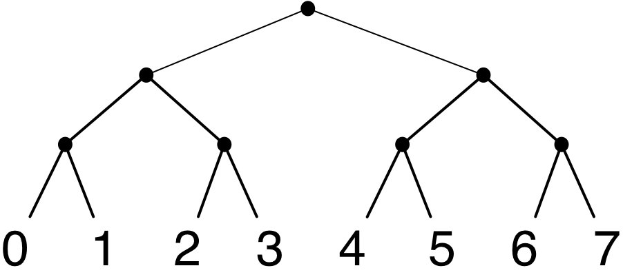
(In a drawing, the depth of a node is the number of edges in a path from the root to that node, and the height of a tree is the maximum depth over all nodes.) If we store values of the sequence at the leaves and use the internal nodes for navigation, we can get to any value in \(O(k)\) time, which is \(O(\log n)\) time if \(n=2^k\).
We can represent an index as a \(k\)-bit binary number and use the bits of an index from most significant (leftmost) to least significant (rightmost) to indicate left child or right child. For example, if \(k=3\):
0 is represented by 000 since \(0=0\cdot 2^2+0\cdot 2^1+0\cdot 2^0\).
1 is represented by 001 since \(1=0\cdot 2^2+0\cdot 2^1+1\cdot 2^0\).
2 is represented by 010 since \(2=0\cdot 2^2+1\cdot 2^1+0\cdot 2^0\).
3 is represented by 011 since \(3=0\cdot 2^2+1\cdot 2^1+1\cdot 2^0\).
4 is represented by 100 since \(4=1\cdot 2^2+0\cdot 2^1+0\cdot 2^0\).
And so on. If we conceptually label each leaf with the index of the value stored there, the leaves are labelled \(0,1,\ldots 2^k-1\) from left to right in a drawing, which is attractive.
Here are some drawings of perfect trees, where instead of labelling leaves with their indices, I have labelled them with the value stored there.
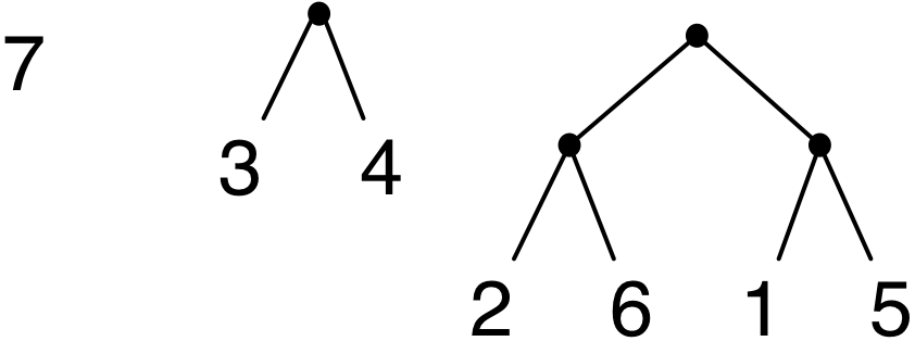
Here is an OCaml data type for such leaf-labelled trees, where the values can be of some arbitrary type. I have also shown the OCaml expressions for the three perfect trees drawn above. The definition does not enforce perfection; the code that manipulates trees has to do that.
type 'a l_bintree = |
Leaf of 'a |
| Node of 'a l_bintree * 'a l_bintree |
|
let ex1 = Leaf 7 |
let ex2 = Node (Leaf 3, Leaf 4) |
let ex3 = Node (Node (Leaf 2, Leaf 6), Node (Leaf 1, Leaf 5)) |
|
let bad = Node (Node (Leaf 8, Leaf 3), Leaf 12) |
The tree called bad is not perfect, since it has some leaves at depth 2 (the ones storing values 8 and 3) and one leaf at depth 1 (the one storing 12). Before we start using perfect trees to try to improve the running time of an implementation of the Sequence ADT, let’s consider the task of determining whether an l_bintree value is perfect or not. Here is a possible solution utilizing the && operator, which is logical OR (does not evaluate right argument if left one is true).
let rec is_perf (t : 'a l_bintree) : bool = |
match t with |
| Leaf _ -> true |
| Node (l, r) -> is_perf l && is_perf r |
This is an incorrect solution, though, as is_perf bad evaluates to true. A perfect tree has two perfect subtrees, but they have to be the same height. That observation yields a recursive characterization of perfect trees: a tree is perfect if and only if it is a leaf or if it has two perfect subtrees of the same height. This can be turned directly into code with the aid of a function that calculates height using structural recursion.
let rec height = function |
| Leaf _ -> 0 |
| Node (l, r) -> 1 + max (height l) (height r) |
|
let rec is_perf = function |
| Leaf _ -> true |
| Node (l, r) -> |
is_perf l && is_perf r && (height l = height r) |
This code is correct, and quite readable, but what is its running time? The running time of is_perf depends on the running time of height. Both of these functions can be applied to arbitrary trees which may not be perfect.
height applied to a tree recursively computes the height of the left and right subtrees. Intuitively, the code does constant work at each node, so the total work should be linear in the number of nodes. Formally, if we define \(T_\mathit{height}(n)\) to be the running time of height on a tree with \(n\) constructors, we get a recurrence that looks like this:
\begin{align*}T_\mathit{height}(1) &= O(1)\\ T_\mathit{height}(n) &= \max_{0 < i < n} \{T_\mathit{height}(i)+T_\mathit{height}(n-i-1)\}+O(1)\end{align*}
We have to use \(\max\) here because we don’t know the number of nodes \(i\) in the left subtree, but we are using worst-case analysis. By strong induction on \(n\), we can show that \(T_\mathit{height}(n)\) is \(O(n)\). (The worst case is a tree where each left subtree is a leaf.)
Although we derived this recurrence for specific code, it is quite general. It will show up whenever code does recursion on both subtrees of a binary tree and the two results can be combined in constant time. Sometimes we know something about the shape of the tree (for example, that it is perfect), but that does not change the solution.
Now we can analyze is_perf. If \(T_\mathit{is\_perf}(n)\) is the running time of is_perf on a tree with \(n\) constructors, we get this recurrence:
\begin{align*}T_\mathit{is\_perf}(1) &= O(1)\\ T_\mathit{is\_perf}(n) &= \max_{0 < i < n} \{T_\mathit{is\_perf}(i)+T_\mathit{is\_perf}(n-i-1) +T_\mathit{height}(i)+T_\mathit{height}(n-i-1)\}+O(1)\end{align*}
Substituting the solution for height, we get:
\begin{align*}T_\mathit{is\_perf}(1) &= O(1)\\ T_\mathit{is\_perf}(n) &= \max_{0 < i < n} \{T_\mathit{is\_perf}(i)+T_\mathit{is\_perf}(n-i-1)\}+O(n)\end{align*}
If the max always occurs at \(i=1\) (again, when each left subtree is a leaf), then we can see that the solution would be \(O(n^2)\). This is in fact the general solution, which can be proved by strong induction on \(n\). This recurrence will also show up a lot, but sometimes we can get a better solution, for example, if the tree is perfect. That doesn’t help us this time, because is_perf can be applied to non-perfect trees.
It shouldn’t take quadratic time to check perfection. The problem is that we are recursively descending into each subtree twice: once to compute the height, and once to verify perfection. Why not do these tasks at the same time, with only one recursion?
We will have is_perf produce an option type which is either Some h when the tree is a perfect tree of height \(h\), or None if it is not perfect.
let rec is_perf (t : 'a l_bintree) : int option = |
match t with |
| Leaf _ -> Some 0 |
| Node (l, r) -> match (is_perf l, is_perf r) with |
| (Some lh, Some rh) -> |
if (lh = rh) then Some (lh+1) else None |
| _ -> None |
Now the recurrence is:
\begin{align*}T_\mathit{is\_perf}(1) &= O(1)\\ T_\mathit{is\_perf}(n) &= \max_{0 < i < n} \{T_\mathit{is\_perf}(i)+T_\mathit{is\_perf}(n-i-1)\}+O(1)\end{align*}
and the solution is that \(T_\mathit{is\_perf}(n)\) is \(O(n)\).
That was more complicated than you might have guessed at the start. Recursive code can be easy to write, but here, we are always concerned with efficiency, and it is also easy to write beautiful but inefficient recursive code. Please keep in mind our primary goal, and examine your code carefully to detect such inefficiencies. Now let’s get back to using perfect trees for sequences.
The perfect binary tree representation only works to store a sequence of length \(n\) when \(n\) is a power of 2. But since any natural number can be expressed as a sum of distinct powers of 2, we can try to use a collection of perfect binary trees of different heights for an arbitrary \(n\). (This can be made to work, and is left as an exercise, specified later.)
In a perfect binary tree of height \(k\) with values stored only at leaves, it takes \(O(k)\) time to access any value, even the one of index \(0\), so this does not work as well as the list implementations for small indices. We can do better for some values by storing values at internal nodes also. In this case, the following type for node-labelled trees is a little cleaner.
type 'a bintree = |
Empty |
| Node of 'a * 'a bintree * 'a bintree |
What is a leaf, in this representation? If we go by what was a leaf in the previous drawings, then a leaf is a Node with two Empty subtrees. But if we think of a leaf as a base case, then a leaf is an Empty constructor. We will use this second interpretation. In drawings, we won’t show Empty constructors (there is no standard visual representation of an empty tree) so you need to keep them in mind.
We’re now restricted to exactly \(n=2^k-1\) values for some natural number \(k\). To fix this while sticking to the idea of using a single tree, we give up on perfection, and use a near-perfect tree, where every leaf is at depth \(k\) or \(k-1\). The number of Nodes is always exactly one less than the number of Empty leaves (this can be proved by induction on the number of constructors).
Besides allowing us to work with arbitrary \(n\), a near-perfect tree gives us some flexibility that we might exploit (by choosing where the gaps are on the lower level of Nodes). The numbering most similar to the attractive numbering of leaves puts the value of index 0 at the root, indices 1 and 2 at left and right child, indices 3, 4, 5, 6 at the next level, and so on. This puts the nodes (or leaves) at lowest depth as far to the left as possible. We might call this a "left-justified near-perfect binary tree" (or LJNP tree).
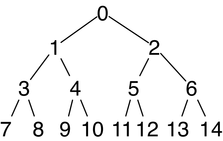
This image shows a perfect tree with 15 nodes. To get one with fewer nodes, say \(n\), we just remove nodes of index \(n\) or higher.
Exercise 2: Give a recursive definition characterizing LJNP trees, and use this to write code that checks whether or not a tree is LJNP. Your code should run in linear time. \(\blacksquare\)
We need a way to compute the path to the value of index \(i\) in a LJNP tree. You can probably work out some indexing algorithm by examining small cases. One clever way of doing the computation is to alter the standard binary representation which represents any natural number with the minimum number of digits, each digit (bit) being either 0 or 1. In standard binary representation:
0 is represented by 0 since \(0=0\cdot 2^0\).
1 is represented by 1 since \(1=1\cdot 2^0\).
2 is represented by 10 since \(2=1\cdot 2^1+0\cdot 2^0\).
3 is represented by 11 since \(3=1\cdot 2^1+1\cdot 2^0\).
4 is represented by 100 since \(4=1\cdot 2^2+0\cdot 2^1+0\cdot 2^0\).
All modern 64-bit architectures store 64-bit integers in two’s complement representation, which coincides with standard binary representation for nonnegative integers. There are consequently two ways of working with bits: modular arithmetic, and bitwise operations. The former is easier to get right, though the latter is faster at the machine level and should be considered for frequently-executed production code. For learning purposes, I would suggest using arithmetic, as it is easier to get right (and to debug when you get it wrong).
In bijective binary numbering, instead of using the digits 0 and 1, we use the digits 1 and 2. They are still used as multipliers for powers of two.
1 is represented by 1 since \(1=1\cdot 2^0\).
2 is represented by 2 since \(2=2\cdot 2^0\).
3 is represented by 11 since \(3=1\cdot 2^1+1\cdot 2^0\).
4 is represented by 12 since \(4=1\cdot 2^1+2\cdot 2^0\).
5 is represented by 21 since \(5=2\cdot 2^1+1\cdot 2^0\).
6 is represented by 22 since \(6=2\cdot 2^1+2\cdot 2^0\).
7 is represented by 111 since \(7=1\cdot2^2+1\cdot 2^1+1\cdot 2^0\).
It’s not hard to show that every positive integer has a unique bijective binary representation and every sequence of digits represents a number. (This is not true when using 0 and 1; we need a convention about omitting leading zeroes.) Furthermore, it’s as easy to figure out the digits in this representation as it is for regular binary, by computing them in reverse order. The least significant digit (rightmost) represents the multiplier for \(2^0\), and the digits to its left represent the multiplier for \(2^1\), \(2^2\), and so on. So the least significant digit is determined by the parity (even/odd) of the number. Non-zero even numbers have least significant digit 2, and odd numbers have least significant digit 1. We can remove the least significant digit by subtracting off that digit value and dividing by 2, and continue to extract the rest of the digits.
We use the bijective binary representation of the index to navigate. The value of index \(i\) is at the root if \(i\) is 0, in the left subtree if the most significant digit of \(i\) is 1, and in the right subtree if the most significant digit (leftmost) of \(i\) is 2. We remove that digit from the index and continue until we have found the value.
Unfortunately, this numbering works fine for first and index, but it’s not at all clear how to efficiently code extend and rest. Even index is a bit messy, since we have to compute and store all the digits of the index (from least significant to most significant) before using them one at a time in the opposite order, starting with the last one we computed. (You might be able to think of ways of computing the most significant digit first, but they’re not going to be as simple.)
Our choice of numbering was arbitrary. We’re allowed to change our mind and use a different numbering if it makes computation easier or more efficient. So let’s try navigating starting with the least significant digit, which is easier to compute. We won’t change the interpretation of 1 as left and 2 as right. This moves the value of index \(i\) to a different position in the tree for some values of \(i\).
It starts out looking like the other numbering, with the value of index 0 at the root, and indices 1 and 2 at left and right child. But the next level has indices 3, 5, 4, 6 in left-to-right order. That doesn’t seem as attractive. But it does make index a bit simpler to code.
Exercise 3: Write OCaml code for index. \(\blacksquare\)
The real payoff, however, is that extend and rest become both simpler to code and clearly efficient. We can see the reason if we fill in the next level in the example.

Again, this image is of a perfect tree; a near-perfect tree with \(n\) nodes only has nodes of index \(0\) through \(n-1\).
The value of index \(2j+1\) (for arbitrary \(j\)) is in the left subtree (since its least significant digit is 1), and the next value, of index \(2j+2\) is in exactly the same position in the right subtree (since its least significant digit is 2, and removing that results in the same value \(j\) for the rest of the navigation).
This means that the right subtree of extend e s is exactly the left subtree of s. This is a huge win, since we don’t have to do any additional computation. The left subtree of extend e s is the right subtree of s, but extended with the element of index 0 in s (since that has index 1 in extend e s). This is a single recursive application of extend.
What we have discovered is that the code for extend makes one recursive call, on the right subtree of its sequence argument, but doesn’t have to do any computation on the left subtree.
Exercise 4: Write the OCaml code for extend. \(\blacksquare\)
If \(T_\mathit{extend}(n)\) is the running time for applying extend to the representation of a sequence of length \(n\), then we get the following recurrence:
\begin{align*}T_\mathit{extend}(0) &= O(1)\\ T_\mathit{extend}(2k+1) &= T_\mathit{extend}(k) + O(1)\\ T_\mathit{extend}(2k+2) &= T_\mathit{extend}(k+1) + O(1)\\\end{align*}
It is possible to come up with an exact solution for this recurrence, but if we first express the recurrence this way:
\begin{align*}T_\mathit{extend}(0) &= O(1)\\ T_\mathit{extend}(n) &= T_\mathit{extend}(\lfloor n/2\rfloor) + O(1)\\\end{align*}
and then remove the use of the floor function, we can come up with a simpler recurrence whose solution for powers of 2 is obvious:
\begin{align*}T_\mathit{extend}(0) &= O(1)\\ T_\mathit{extend}(n) &= T_\mathit{extend}(n/2) + O(1)\\\end{align*}
Applying Akra-Bazzi, the solution to the general recurrence is that \(T_\mathit{extend}(n)\) is \(O(\log n)\). We could also argue that the running time of extend is \(O(k)\), where \(k\) is the height of the tree representing the sequence argument, and \(k = O(\log n)\) where \(n\) is the length of the sequence. But each of these are just imprecise versions of the (itself imprecise) above recurrence relation.
Exercise 5: Complete the implementation of Sequence using Braun trees. Show that the analysis of rest involves a recurrence similar to that of extend, and that the solution is also \(O(\log n)\), where \(n\) is the length of the sequence. \(\blacksquare\)
Exercise 6: Work out the algorithm and the OCaml code for a new operation, update, which consumes an index and a value, and produces a new version of the sequence with the element at the given index updated to be the provided value. Show that this code also runs in logarithmic time. \(\blacksquare\)
The data structure we have derived is called a Braun tree, after its inventor, and dates from 1983. The exercises above show that Braun trees can be used in a purely-functional simulation of arrays, but with access cost that is logarithmic instead of constant (and with the ability to grow/shrink at much lower cost than for arrays).
A Braun tree with \(2k+1\) nodes has two subtrees with \(k\) nodes (the ones of odd index and the ones of nonzero even index) and both subtrees are also Braun trees. A Braun tree with 2k+2 nodes has a left subtree with \(k+1\) nodes (the ones of odd index) and a right subtree with \(k\) nodes (the ones of nonzero even index), and both subtrees are also Braun trees. We can make this into a recursive definition: a Braun tree is either empty, or it has two Braun subtrees either with equal number of nodes or the left one has one more node.
Exercise 7: Write OCaml code to check whether or not a tree is a Braun tree. Your code should run in linear time. \(\blacksquare\)
If we define \(T_\mathit{index}(i,n)\) to be the running time of index with index argument \(i\) and sequence argument of length \(n\), we have the following recurrence (again neglecting floors and ceilings):
\begin{align*}T_\mathit{index}(i,0) &= O(1)\\ T_\mathit{index}(0,n) &= O(1)\\ T_\mathit{index}(i,n) &= T_\mathit{index}(i/2, n/2) + O(1)\\\end{align*}
The solution to this is \(T_\mathit{index}(i,n) = O(\min\{\log i, \log n\})\). Intuitively, each parameter is reduced by a factor of 2 at a constant cost, so the total cost is proportional to the logarithm of the first parameter to reach 0, that is, the smaller parameter. This is a considerable improvement over the list-based implementation, which was our original motivation.
We can see that the Braun tree implementation of sequences is not better in all cases than the list implementation. Lists have \(O(1)\) implementations of rest and extend, while Braun trees take \(O(\log n)\) time. But Braun trees do better on index. It is possible, with a different idea, to lower the cost of rest and extend to \(O(1)\), while preserving the \(O(\log n)\) part of the cost of index.
Consider the effect of applying the update operation (defined in the exercise above) to a Braun tree. The shape of the new tree is exactly the same as the shape of the old tree, and the only difference in values is at the index that was updated. But the cost is only logarithmic in the index. What does the sharing look like between the new tree and the old tree?
A little thought will convince you that there is a new version of every node on the path from the root down to and including the node containing the value to be updated (so the new space is logarithmic in the index). Every new node has one subtree shared with the old tree (the branch not taken) and one subtree with another new node as root (corresponding to the next node on the path) except the node containing the value being updated, which has both subtrees (if not empty) shared with the old tree. This is called "path copying" when considered from the point of view of imperative implementations that need to add some persistence. It happens naturally in a functional implementation.
The Braun tree is not a data structure that is widely used in practice. It is, however, well-suited for a pedagogical exposition of some of the issues that repeatedly arise in the study of data structures, and we will see it again later on.
Exercise 8: Write OCaml functions to convert between the Braun tree representation of a sequence and the list representation of a sequence. Each function should run in linear time. Hint: in the forward direction, process the tree in a top-down, breadth-first (level-by-level) manner, and in the reverse direction, build the tree bottom-up and level-by-level. \(\blacksquare\)
Exercise 9: Write OCaml code that uses a list of binary digits in order from least significant to most significant to represent a natural number, with the following interface, where inc and dec add one and subtract one respectively.
type digit = Zero | One |
type nat = digit list |
|
val zero : nat |
val is_zero : nat |
val inc : nat -> nat |
val dec : nat -> nat option |
\(\blacksquare\)
Exercise 10: A PBLT is not a hybrid of the PBJ and BLT sandwiches (which would be a PBJLT, and probably not very good) but a list of perfect binary trees with elements at the leaves, where the tree of list index \(i\) (counting from zero) is either a tree with \(2^i\) leaves or an empty tree. The representation of an empty sequence is an empty list.
Using the fact that every number has a unique representation as a sum of distinct powers of 2 in standard binary notation, we can represent any sequence as a PBLT using the front-to-back ordering of lists and, within a tree, the left-to-right ordering of leaves. A tree with \(2^i\) leaves corresponds to a 1 digit multiplying \(2^i\) in the binary representation, and an empty tree corresponds to a 0 digit.
Complete an OCaml implementation of the Sequence ADT using PBLTs, conforming to the following signature.
type 'a tree = Leaf of 'a | Node of int * 'a tree * 'a tree |
type 'a digit = Zero | One of 'a tree |
type 'a sequence = 'a digit list |
The extra information in the Node constructor for a nonempty tree (the first field, before the left and right subtrees respectively) is the number of leaves. Although this number is determined by location in a PBLT, it is convenient to maintain it, rather than compute it when needed.
Analyze your implementation. You should find that PBLTs come close to Braun trees, but some operations do worse. \(\blacksquare\)
Exercise 11: Redo the earlier binary digit implementation exercise, but with bijective binary numbering instead.
type digit = One | Two |
type nat = digit list |
|
val zero : nat |
val is_zero : nat |
val inc : nat -> nat |
val dec : nat -> nat option |
\(\blacksquare\)
Exercise 12: Redo the earlier implementation of the Sequence ADT using PBLTs, but using bijective binary numbering instead.
type 'a tree = Leaf of 'a | Node of int * 'a tree * 'a tree |
type 'a digit = One of 'a tree | Two of 'a tree * 'a tree |
type 'a sequence = 'a digit list |
Analyze your implementation. You should find that none of the operations gets worse in O-notation terms, compared to the earlier implementation, and at least one gets better. \(\blacksquare\)