4 Sets and Maps
\(\newcommand{\la}{\lambda} \newcommand{\Ga}{\Gamma} \newcommand{\ra}{\rightarrow} \newcommand{\Ra}{\Rightarrow} \newcommand{\La}{\Leftarrow} \newcommand{\tl}{\triangleleft} \newcommand{\ir}[3]{\displaystyle\frac{#2}{#3}~{\textstyle #1}}\)
"I sleep in the daytime / I work in the nighttime / I might not ever get home"
Talking Heads, "Life During Wartime", Fear of Music, 1979
This chapter discusses two important abstract data types. The Set ADT defines a computational version of the mathematical notion of set. It is parameterized on the type of element in the set, and supports operations such as element-of, union, intersection, and set minus. The Map ADT is also known as Table, Dictionary, or Associative Array. It provides an interface that describes finite maps from some domain to some range, so it is parameterized on two types. The operations include lookup, add, and remove. Implementations for most modern programming languages are either part of the syntax or provided in the standard library. Elements of the domain are called keys; a key maps to an associated value (which I abbreviate as "avalue", but no one else does) in the domain.
A single implementation idea can often be applied to implement both of these ADTs. If a value in an implementation of the Set ADT is stored in its entirety (as is the case, for example, in a Braun tree implementing Sequence), then we can consider it as a key and also store the associated avalue with it. This will be the case for most of the implementations in this chapter, and so we will focus on Set. But not every implementation of the Set ADT stores entire set values or keys. For example, a bitmap (a sequence of bits where each bit represents the presence or absence of some key) has only an indication that a key is in a represented set, and it would take some work to store avalues.
Given an implementation of the Map ADT, we can store sets by simply making the avalue some dummy value. But the Map ADT does not have equivalents of union and intersection, and these operations may be expensive to add to some implementations. We saw this phenomenon with some implementations of Priority Queue in Chapter 3, where we needed a new idea to implement merge. In the implementations described here, we will be able to achieve good performance on union, intersection, and set difference.
4.1 Ordered domains
With priority queues, the ordering of stored values was an important part supplied by the user. In our implementations of Set, we will make use of an ordering on the domain, but it does not have to be supplied by the user. It is only used to help deliver the promised efficiency. Some domains do not have a "natural" ordering, or the natural ordering is not really relevant. But for most domains, one can create some ordering that suffices.
Although points in the two-dimensional plane do not have a natural ordering, we can impose one: compare the x-coordinates, and if one is smaller, that point is smaller. But if they are the same, compare the y-coordinates. This can generalize to arbitrary tuples (comparing from left to right), and to unbounded sequences like lists. In the case of different lengths, if one sequence is a prefix of another, the shorter one is considered to be smaller. This ordering is called lexicographic, because it is the ordering of words in an English dictionary (considering the words as sequences of letters). It is useful enough that some languages provide predefined ways of using it. Haskell has the Ord typeclass that can be automatically derived for many datatypes. OCaml has a generic compare operation that provides a similar functionality, and the structural ordering functions (<, >, <=, >=).
For any given domain, we can fix an ordering to use in our algorithms. In Chapter 3, I discussed general mechanisms involving functors that let one provide an arbitrary ordering for use by generic code. The OrderedType datatype described there is used by the OCaml library modules Set and Map. For simplicity, in this chapter I will assume keys are compared using the structural ordering functions, but you should feel free to write fully general code for the exercises, if you’d like the practice.
4.1.1 Binary search trees: the naive implementation
In a Map, there can be at most one value associated with a key, and in a Set, there can be at most one occurrence of a key. All the implementations we discuss in this chapter can be easily adapted to handle multisets, where there can be several occurrences of the same value.
The operations for Map are empty, lookup, insert, and delete. The operations for Set are empty, is_empty, member_of, subset_of, union, intersection, and difference (set minus). These operations alone do not permit one to build nonempty sets. The more mathematical approach is to add an operation that creates a singleton set from one element. On the computer science side, algorithmic applications often make use of insert and delete operations for Set.
We will focus on binary search trees (BSTs), which you may have encountered in your earlier exposure to programming. If not, don’t worry, we will start from scratch. A binary search tree is a binary tree that satisfies an additional property or invariant known as the BST property. We can keep in mind the binary tree data type we developed in Chapter 2.
type 'a bintree = |
Empty |
| Node of 'a * 'a bintree * 'a bintree |
The BST property is that all the elements in the left subtree are less than the root (using the domain ordering we have decided to use), those in the right subtree are greater than the root, and the two subtrees are (recursively) binary search trees. As with heaps, there are many possible representations for a given set of keys.
Exercise 29: Draw all six binary search trees for the set \(\{1,2,3\}\). \(\blacksquare\)
Exercise 30: Write an is_bst function that runs in linear time. Think carefully about what information needs to be passed in parameters of a helper function, and what information is produced by a recursive application. \(\blacksquare\)
We will start by discussing the simplest "naive" implementation sometimes used in early programming courses. The element_of operation testing whether a given domain value is an element of a represented set (also known as lookup or search) uses structural recursion on at most one subtree (or neither, if the given value is at the root) and consequently takes \(O(h)\) time, where \(h\) is the height of the tree. This operation does not change in more sophisticated implementations.
Exercise 31: Write OCaml code for element_of. \(\blacksquare\)
The height of the tree depends on the implementation of insert and delete. Naive insertion also uses structural recursion on at most one subtree, and the result is that the new tree looks like the old tree, except that an Empty leaf of the old tree has been replaced by a Node containing the new element. The Empty leaf is exactly where a lookup of the new element in the old tree would fail.
Exercise 32: Write OCaml code for naive insert. \(\blacksquare\)
Unfortunately, naive insertion can result in a tree with \(n\) nodes that has height \(O(n)\). Inserting keys in increasing order gives a tree with no nonempty left subtrees, essentially a list. Naive deletion (which is a little more complicated) can have a similar effect. Deletion of a value at a node with one or two empty children is easy; a value at a node with two nonempty children can be replaced by the largest value in its left subtree, which will be at a Node with two Empty children and so can be easily moved.
Exercise 33: Write OCaml code for naive delete. \(\blacksquare\)
These algorithms are easiest to describe and justify in a purely-functional fashion, meaning a persistent implementation of an immutable ADT. But they can also be implemented using mutation and loops, giving an ephemeral implementation of a mutable ADT, and that is what many popular textbooks and courses do. We will not need to use mutation in this chapter.
Both immutable and mutable implementations make for nice small programming exercises, but from a worst-case point of view, we might as well use lists, which results in even simpler code. We need to use more clever algorithms to reduce the height of produced binary search trees, without taking too much time.
4.1.2 History of efficient implementations
There are limits to how well we can do using binary search trees. In Chapter 3, we saw how to flatten a leaf-labelled tree in linear time. If we do this for a BST, but place the root value between the sequences generated by flattening left and right subtrees, the result is a sorted sequence of keys, obtained with no further comparisons. Since we can create a BST holding \(n\) keys with \(n\) insert operations, but we cannot sort these keys in \(o(n \log n)\) time, a comparison-based BST implementation cannot reduce the cost of all operations to \(o(\log n)\).
We say a binary tree with \(n\) nodes is balanced if its height is \(O(\log n)\). The implementations we will study achieve this, and will do so while taking time \(O(\log n)\) for operations producing new trees. These algorithms take the form of stating an additional invariant which can be shown to guarantee logarithmic tree height, and which can be maintained by operations within the desired running time.
In Chapters 2 and 3, we saw binary trees with these height bounds. But the near-perfect trees we used for sequences and priority queues (left-leaning and Braun) do not seem to help for Set operations. There is only one shape for a given number of nodes, and, given a set of keys, this dictates the position of every key. This doesn’t allow enough flexibility to insert and delete efficiently. Allowing all near-perfect trees gives more possibilities, but it is unclear how to take advantage of them. In other words, the invariants we used earlier are not good enough.
The first implementation of a balanced BST for Map was AVL trees, published in 1962 in a Soviet journal. Delightfully, the acronym does not abbreviate three words or three authors, but two authors, Adelson-Velsky and Landis. AVL trees, as we will see, use a height criterion similar to the depth criterion for near-perfect trees.
Bayer and McCreight, in 1970, investigated non-binary perfect trees, where all leaves were at the same depth but flexibility was provided by possibly storing more than one key in a node. Nievergelt and Reingold, in 1973, used a weight (size) criterion to balance trees. Guibas and Sedgwick, in 1978, found an ingenious way to encode a certain kind of non-binary perfect tree into a binary tree, and gave their data structure the name "red-black tree". Aragon and Seidel, in 1989, combined the BST property with the heap property (not on keys) to create "treaps". These have perhaps the simplest implementation among the ones we’ll discuss, because balance is achieved with the use of randomization (so results are "with high probability").
For a Standard ML competition in 1993, Adams found an elegant, purely-functional implementation of sets using weight-balanced trees. Blelloch and Reid-Miller adapted this for treaps in 1998, considering a parallel setting where more processors can be used to reduce the time while keeping work the same (within a constant factor). Blelloch, Ferizovic, and Sun extended this work in 2016 to include AVL, weight-balanced, and red-black trees.
These last three papers provide the general framework that we will use to discuss these four balancing methods (though I will only once point out an opportunity for parallelism, and not discuss its analysis).
4.1.3 The general framework
To recap, we are pursuing a general method of implementing treaps, AVL trees, weight-balanced trees, and red-black trees that emphasizes their common aspects. A conventional presentation tends to focus on insert and delete. At least initially, these can be viewed as modifications of naive insert and delete. The location of the change is found by recursively descending into the BST, where imbalances created by the operation are corrected "on the way back" from the recursion. This view can be obscured if recursion is replaced by loops, and other optimizations are implemented.
In the framework used here, there is only one helper function, join, that is specialized for each of these implementations; every other helper function or operation is derived and can be implemented generically (identically for all four implementations). The analysis is also generic once certain key properties of the join implementation have been established.
The join operation consumes three arguments \(L,k,R\), where \(L\) and \(R\) are BSTs with the property that all keys in \(L\) are less than \(k\), and all keys in \(R\) are greater than \(k\). It produces a BST containing all keys in \(L\) and \(R\) as well as \(k\). Each implementation of join makes sure that the specific invariant for that BST version is satisfied by the result, assuming that it is satisfied by \(L\) and \(R\). The remaining functions, being generic, do not have to worry about what invariant is being maintained.
If the join operation did not have to worry about the version invariant, and just had to ensure the BST property, it would be nothing more than the Node constructor. We can think of the join operation as being a "smart" version of the Node constructor that knows about the additional invariant.
We will discuss the four specific implementations of join later. First, let’s derive the other operations.
We start with a useful helper operation split, which consumes a key \(k\) and a BST \(T\). It produces a triple \((L,b,R)\), where \(L\) is a BST with all keys less than \(k\), \(R\) is a BST with all keys greater than \(k\), and \(b\) is a Boolean value that is \(\mathit{true}\) if and only if \(k\) is in \(T\). This operation is a little harder to motivate before seeing its use. It represents a common action of deconstructing a BST into pieces that can then be reassembled in a different way to ensure the version-specific invariant. You are familiar with separating \(T\) into the root key and the left and right subtrees in the course of structural recursion. If \(k\) is the root key, then split is trivial. The interesting case is when it is not the root key.
The base case of split is if \(T\) is Empty, in which case the result is (Empty, false, Empty). Otherwise \(T\) is a tree with root \(r\) and left and right subtrees \(L',R'\). We compare \(r\) to \(k\), with three outcomes. If they are equal, the result is \((L',\) true\(,~R')\). If \(k < r\), then we need to recursively split \(L'\) using \(k\) into \((L'',b,R'')\) and then form the result \((L'',b,\mathit{join}~R''~r~R)\). The remaining case is symmetric.
Using these two helper functions, we can implement the ADT operations. I hope you will agree, once you complete this task, that it is is not challenging, in the sense that there are clever ideas used. It’s just a matter of using the tools at hand.
Let’s start with insert. We didn’t list this as a Set operation, but we can consider it as "union with a singleton set", which might be easier than general union. (One of the annoying differences between math and CS is that there is no concise math notation for this operation, which is more common in CS.) To insert \(k\) into \(T\), we split \(T\) into \((L,b,R)\) using \(k\), and then join \(L\) and \(R\) using \(k\). (What role does \(b\) play?)
The delete operation is left as an exercise for you, with a hint to first look back at naive deletion and then to write and use the following helper functions. find_max and delete_max pretty much do what their name says (delete_max produces a pair of the deleted element and the new tree), and join2 is like join, but without the middle element.
To form the union of nonempty \(T_1\) and \(T_2\), we split \(T_1\) into \((L,b,R)\) using the root of \(T_2\). We recursively form the union of \(L\) and the left subtree of \(T_2\), and similarly the union of \(R\) and the right subtree of \(T_2\). (These two recursions could be done in parallel, if we were considering a parallel setting.) Then we join these using the root of \(T_2\). If \(T_2\) is a singleton set, this code reduces to what we did for insert, meaning that we didn’t really gain much by making it a special case. The intersection and difference operations are left as exercises for you. These have a similar structure to union and similar opportunities for parallelism.
The memberOf operation can be implemented by splitting and producing the Boolean value, ignoring the two BSTs produced. (Or directly by the naive lookup function.) The subsetOf operation can be implemented using difference.
The split and join operations as components of implementations of Set using balanced binary trees go back as far as a series of lectures by Tarjan in 1981, though he seems to have not noticed (or cared) that they could be used for insert and delete, because he treated these separately.
Clearly, the analysis of these depends on the implementation and analysis of join. We will tackle that starting in the next section.
Exercise 34: Provide an OCaml implementation of the above derived functions, conforming to this signature:
module type bst_impl = sig |
type 'a bst |
val empty : 'a bst |
val unwrap : 'a bst -> ('a * 'a bst * 'a bst) option |
val join : 'a bst -> 'a -> 'a bst -> 'a bst |
end |
|
module type bst_deriv = sig |
|
module BSTImpl : bst_impl |
|
type 'a bst = 'a BSTImpl.bst |
|
val split : 'a -> 'a bst -> 'a bst * bool * 'a bst |
val is_empty : 'a bst -> bool |
val insert : 'a -> 'a bst -> 'a bst |
val find_max : 'a bst -> 'a option |
val delete_max : 'a bst -> ('a * 'a bst) option |
val join2 : 'a bst -> 'a bst -> 'a bst |
val delete : 'a -> 'a bst -> 'a bst |
val union : 'a bst -> 'a bst -> 'a bst |
val intersect : 'a bst -> 'a bst -> 'a bst |
val diff : 'a bst -> 'a bst -> 'a bst |
end |
|
module BSTDeriv (I : bst_impl) : (bst_deriv with module BSTImpl = I) |
The unwrap function exposes the tree structure by providing the root value and left and right subtrees; this will be useful to you in writing some of the derived functions in a generic fashion, and you can also use it for white-box testing.
Your implementation of find_max should use structural recursion; insert, delete_max, join2, and delete should not use recursion directly (they apply other functions that may use recursion). The cost of each function should be dominated by the cost of join and split (which we will analyze later).
You will need an implementation of join to test your code. One possibility is to simply use the Node constructor; a better one is to use one of the efficient implementations of join discussed below. \(\blacksquare\)
4.1.4 Treaps
We start with treaps because their code is simplest. This is partly because they are the most recent of the variations and thus had the benefit of earlier work, and partly because they use randomization, which allows the code to be simpler at the expense of making the analysis more complex (and the algorithm no longer deterministic worst-case). The implementation is technically not purely functional, because a function generating a random number is not pure (it will not produce the same value if evaluated with the same arguments). However, the randomization in this case does not enter into the correctness arguments; this is not an algorithm with a small error probability. We deal with the randomization only in the analysis of running time.
The basic idea is to add the heap property to a binary search tree. We cannot add the heap property on keys and also preserve the BST property. What we do is pair each key with an associated priority, and enforce the heap property on those priorities. The priorities represent added structure imposed on the BST.
The following observation shows that all the possible flexibility of rearranging the BST has been moved into the choice of priorities: if all the priorities associated with a set of keys are distinct, then there is only one BST that has those keys and associated priorities.
To see this, consider what has to be at the root: the key whose associated priority is smallest. But that key determines the set of keys in the left subtree, and the set of keys in the right subtree. And then we independently repeat the reasoning for those two subtrees. (This is an informal statement of a proof by strong induction on the number of keys.)
Given that we argued that flexibility in tree shape was the key to efficient algorithms, and that near-perfect trees did not offer enough flexibility, you might think that some elaborate scheme to change priorities is coming. But that is not the case. A key is assigned a priority once, when it is inserted, and never changed. That is what makes the code so simple; it looks at priorities but never modifies them. The final idea remaining is the choice of priorities, and the policy is brilliantly simple: each priority is an independent random number.
We can think of this number as a real number uniformly distributed over the interval \([0,1]\), though in practice we do not have real numbers and we have to either choose a random floating-point number in this range, or use a random 64-bit word treated as an unsigned integer. Choosing two identical random numbers is a probability-zero event in the theoretical view, but a non-zero (but very small) probability event in practice. The effect is to possibly increase the height of the tree by one, slightly increasing the running time, rather than to break any of the algorithms.
Perhaps the brilliance of this choice cannot be fully appreciated until one has tried to analyze a randomized algorithm. The issue is that it is relatively easy to deal with independent random variables, but not so easy to deal with dependent ones. A randomized algorithm is deterministic most of the time, but at some point it generates a random value (say, it flips a coin). Presumably it acts on this value, otherwise there would be no point in the flip. So in the two computational paths that result from the first flip, different things are done. An analysis of the running time will need to consider how many steps are taken in various tasks within the algorithm. Those measurements become random variables, but the random variables are not independent; they may depend on the outcomes of the same coin flip. And that dependency is hard to deal with.
The definition of two events \(E_1\) and \(E_2\) being independent is if \(\mathit{Pr}[E_1 \mbox{ and } E_2]=(\mathit{Pr}[E_1])(\mathit{Pr}[E_2])\). Consider the following simple example. You flip a coin some large odd number of times \(n\), and count the heads and tails. Intuitively, the probability of the number of heads being much larger than the number of tails is very low, and this can be proved. Now you ask a friend to repeat the experiment, but your friend is lazy. They just flip a coin once and then say that all the other flips produce the same outcome.
Your first flip and your second flip are independent. But your friend’s reported first flip and their reported second flip are not independent; they are dependent. The probability that both are heads is not \(1/4\); it is \(1/2\). This is true despite the fact that the reported second flip, by itself, looks like a legitimate coin flip: it is heads with probability \(1/2\) and tails with probability \(1/2\). Because of the dependency, the probability that the number of heads is much larger than the number of tails is not low for your friend’s experiment; it is \(1/2\).
In general, if we want to say something about the state of a randomized algorithm partway through its work, that will depend on the history of how it got to where it is. In the case of data structures that employ randomization, the sequence of operations usually has to be taken into account. But that is not the case for treaps. The uniqueness property ensures that history does not matter; the tree is determined entirely by the set of keys and their associated priorities. This simplifies the analysis.
Let’s reason about how to join two treaps \(L\) and \(R\) with key \(k\). We find the smallest priority among \(k\) and the roots of the two trees. If the smallest priority is associated with \(k\), we just use the Node constructor. If the smallest priority is associated with the root of \(L\), that must be the root of the result. The left subtree of the result will be the left subtree of \(L\), and the right subtree of the result will be the recursive join of the right subtree of \(L\), \(k\), and \(R\). The third case is symmetric.
What remains is to analyze the running time of join, and then the derived operations. Since the recursive applications always join using \(k\), the running time is \(O(d)\), where \(d\) is the depth of node \(k\) in the result. The original paper on treaps showed that the running time of the Map operations on a treap with \(n\) nodes is \(O(\log n)\) with high probability. I will show a weaker result, that the expected depth of a node, and consequently the expected running time of the operations, is \(O(\log n)\).
Intuitively, why would this be the case? The proof above that treaps are unique shows that one can view a treap built by operations as having been created by naive insertion in order of priority, and thus by naive insertion in random order. The chance that the split is close to even, say no worse than one-third / two-thirds, is pretty good. We know if the split is always as close to even as possible, we get logarithmic depth (example: a Braun tree). This is still true for a "close to even" split. That is not a proof, and probabilistic analyses can be counter-intuitive. But in this case, the intuition is correct.
Exercise 35: Write OCaml code to implement treaps that fits into the uniform framework. You will need to find out how OCaml deals with random numbers. The derived operations cannot be completely generic, because insert has to assign a new random priority to the inserted element (if it is not already in the set). To aid in testing, you should write a is_treap function that runs in linear time. \(\blacksquare\)
Treaps are quite elegant, but not often used in practice. One reason seems to be their relative obscurity. Indeed, they were independently invented by Vuillemin in 1980, under the name "Cartesian trees" (because of an application involving points in the Cartesian plane). They show up in exercises in a couple of textbooks. Another barrier might be the overhead of generating and maintaining the random numbers involved. The original presentation of treaps, like most presentations of BST variations, was built around insert and delete rather than join and split, and was described in ephemeral imperative terms rather than in a persistent functional manner. Such presentations tend to use rotations, which we will need for the remaining three implementations, but which are not necessary to implement join for treaps.
4.1.4.1 Probabilistic analysis of treap Map operations
The weaker result I said I would prove about treaps requires only a few basic facts about probability, but it still should be considered optional reading, especially if you have had little or no exposure to probability.
The expectation of a random variable is its average, weighted by probability. If the random variable \(X\) can take on values from some domain \(\cal D\), then its expectation \(E[X]\) is defined as \(\sum_{v \in \cal D} v~Pr[X=v]\). (The sum is replaced by an integral if real numbers are involved.) For example, if you win a dollar if a fair flipped coin turns up heads, and nothing if it turns up tails, your expected win is half a dollar, since \(0(1/2)+1(1/2)=1/2\). The key fact we will need about expectations is that they add, that is, for two random variables \(X\) and \(Y\), \(E[X+Y]=E[X]+E[Y]\). This is just an exercise in rearranging summations (or integrals), and it holds for any two random variables, regardless of whether or not they are independent.
Since it is only the relative ordering of the keys that is important, let’s assume the keys are are \(0\) through \(n-1\). This makes the notation simpler. The priorities are still chosen by independent samples of the uniform distribution over \([0,1]\).
Treap Depth Lemma: The expected depth of \(j\) in a treap is \(H_{j+1}+H_{n-j}-2\), where \(H_k=\sum_{d=1}^k(1/d)\) (these are often called "harmonic numbers").
This is a messy expression, but we can bound \(H_k\) above by \(\lceil \log_2 k \rceil\), since \(H_k\le\sum_{i=0}^{\lceil\log_2 k\rceil}\sum_{j=1}^{2^i}(1/2^i) \le\sum_{i=0}^{\lceil\log_2 k\rceil}1=\lceil\log_2 k\rceil\). (A more careful analysis improves the base of the logarithm to \(e\), that is, \(H_k\) is close to \(\ln k\) for large \(k\).) So if we can prove the Treap Depth Lemma, we can say that the expected depth of a particular key in a treap with \(n\) nodes is \(O(\log n)\). Proving it requires the following result.
Treap Ancestor Lemma: \(i\) is an ancestor of \(j\) (for \(i<j\)) in a treap if and only if the priority of \(i\) is smaller than the priorities of \(\{i+1,\ldots,j\}\).
We prove the Treap Ancestor Lemma by induction on the size of the treap. Let \(r\) be the root of the treap. If \(i=r\), then all \(j\) such that \(i<j\) are descendants, and they all have have greater priority, so the statement holds. If \(j=r\), then no \(i\) such that \(i<j\) are ancestors, and they all have greater priority, so the statement holds. If \(i\) is in the left subtree of \(r\) and \(j\) is in the right subtree of \(r\), then \(i<r<j\), there is no ancestor relationship between \(i\) and \(j\), and \(r\) has smaller priority than \(i\), so the statement holds. Finally, if \(i\) and \(j\) are in the same subtree of \(r\), we apply the induction hypothesis.
Having proved the Treap Ancestor Lemma, how do we prove the Treap Depth Lemma? Since the priorities are independent and identically distributed, the probability that \(i\) (where \(i>j\)) is an ancestor of \(j\) in a treap is \(1/(i-j+1)\), since this is the probability that \(i\) has the smallest priority in the set \(\{i,\ldots,j\}\).
We define \(I_{i,j}\) to be 1 if \(i\) is an ancestor of \(j\) and 0 otherwise. (This is known as an indicator variable.) Then the depth of \(j\) is \(\sum_{i \ne j} I_{i,j}\). From the observation in the previous paragraph, the expected value of \(I_{i,j}\) is \(1/(|j-i|+1)\).
So the expected depth of \(j\) is \(\sum_{i \ne j}(1/(|j-i|+1))\), which is \(H_{j+1}+H_{n-j}-2\). Here we are using the fact that the expectation of a sum is the sum of the expectations, and then splitting the sum into the two cases \(i < j\) and \(i > j\). That proves the Treap Depth Lemma, and its corollary that the expected depth of a particular key in a treap with \(n\) nodes is \(O(\log n)\).
How do we show that this holds with high probability and not just in expectation? The Treap Ancestor Lemma shows that if we fix \(i\), the set of indicator variables \(I_{i,j}\) for \(j>i\) are independent, and similarly the set \(I_{j,i}\) for \(j<i\). We can then apply bounds known as Chernoff bounds to the sum in the Treap Depth Lemma which bounds the depth of a node.
A Chernoff bound applies to the sum of independent, identically-distributed random variables. For example, we could use one to be precise about our intuition that in our coin-flipping experiment, the difference of the number of heads and tails will not deviate too far from zero, with high probability. Chernoff bounds are commonly used in the analysis of randomized algorithms.
The fact that the depth of a given node is \(O(\log n)\) with high probability allows us to show that the height of a treap (the maximum depth over all nodes) is \(O(\log n)\) with high probability. We could not do this with just our work on expectations, as \(E[\max\{X_i\}]\) is not necessarily \(\max\{E[X_i]\}\).
Lookup of a key that is in the treap takes time proportional to the depth of the key, which is \(O(\log n)\) (in expectation and with high probability). What about a key that is not in the treap? Continuing with the above notation for keys, a search for a key less than 0 terminates at 0, and a search for a key greater than \(n-1\) terminates at \(n-1\). A search for a key in \((k,k+1)\) terminates either at \(k\) or \(k+1\), and the max of these is bounded by twice the sum, so this is also \(O(\log n)\) with high probability.
As mentioned above, join involving a key \(k\) takes time proportional to the depth of \(k\) in the result, so this is also \(O(\log n)\) with high probability.
A split with key \(k\) behaves like a search for \(k\) (whether successful or unsuccessful) with respect to the recursive splits on the way down. However, the work done after the recursive split amounts to a join at each level moving back up the tree. If we don’t look carefully, and charge \(O(\log n)\) for each join, we conclude that split takes \(O(\log^2 n)\) time. Fortunately, when we do look carefully, we see that the key in each join is the root of the originally split tree, and the other arguments to the join are trees whose keys are subsets of the originally split tree. That means that the priority of the join key is less than the priorities of the roots of the two join arguments, and in this case the join takes \(O(1)\) time. So the work done by all the joins is also \(O(\log n)\) with high probability. Similar reasoning works for the other Map operations.
Exercise 36: If you did the OCaml implementation of the derived Map operations, verify that your code for each operation runs in time \(O(h)\), where \(h\) is the height of the BST, assuming that this is true for join and split. \(\blacksquare\)
4.1.4.2 Remarks on the analysis of set operations
The set operations are more complicated to analyze. We will not achieve logarithmic time, and it’s important to understand why, which is that we can’t hope for this while using BSTs. Consider taking the union of two sets of size \(n\) and \(m\) respectively, where \(m \le n\). Since we are using BSTs, we can recover sorted order for each set separately with no further comparisons, and sorted order for their union (once it is computed) with no further comparisons. What does this say about the number of comparisons needed to do the union?
If all keys are distinct, we can describe the sorted order of the union by specifying which \(m\) positions out of \(n+m\) are occupied by keys from the smaller set. Thus there are \({n+m} \choose m\) possibilities. The same argument we used for the lower bound for comparison-based sorting tells us we have to do at least \(\log_2 {{n+m} \choose m}\) comparisons, which is at least \(\log_2 \left(\frac{n}{m}+1\right)^m\), which is at least \(m\log_2 (\frac{n}{m}+1)\).
So we can’t hope to do better than this. Fortunately, the generic version of union, when used with the specific join for treaps, takes \(O(m \log (\frac{n}{m} +1))\) expected time. The analysis is quite complicated, and there are no known corresponding "with high probability" results. The same time bounds hold for worst-case analysis of the set operations for the other three implementations below.
If we just take the elements of the smaller treap and insert them one at a time into the larger treap, we could achieve \(O(m \log n)\) time. But when \(m\) is about equal to \(n\), \(O(m \log (\frac{n}{m}+1))\) is better, as it is linear in the number of keys. At the other extreme, when \(m\) is one, this analysis suggests that generic union takes \(O(\log n)\) time, which is comparable to generic insert.
Although the analysis of union is too complicated to be done completely here, I can sketch the intuition behind it.
union takes the root of the second tree and uses its key to split the first tree. The recursive calls to union then split the left and right pieces of the first tree with the left and right children of the root of the second tree. Eventually all keys of the second tree are used to split the first tree. If the second tree is smaller, then the splitting produces \(m+1\) pieces. Let’s assume that the second tree is perfect and the pieces have size \(n_i>1\). If we assume that the cost of one split is \(\log n_i\), then the total cost is \(\sum_i \log n_i\). Since \(\log n_i + \log n_j \le \log \frac{n_i+n_j}{2}\) (you should be able to prove this), this sum is greatest when the \(n_i\) are equal, that is, when they are about \(\frac{n}{m}\), making the total cost something like \(O(m \log \frac{n}{m})\).
But the cost of one split is not \(\log n_i\). It is one more than this for the splits done with the leaves of the second tree, two more for their parents, and so on. The cost we neglected is like the cost of linear-time heapify on Braun heaps or array-based heaps. If we heapify \(m\) elements, there is one meld costing \(\log m\), two costing \((\log m)-1\), and so on, and the sum is \(O(m)\). The same idea shows that the cost we neglected was \(O(m)\).
The first tree is not necessarily going to be perfect, but it will have height \(O(\log m)\) with high probability, and the analysis above can be extended to that situation, with a bottom-up definition of layers to be added in the imperfect but balanced tree. We need the size of layers to be geometrically decreasing as we move up the tree, while the cost associated with a node in a layer is linearly increasing, as above. If the first tree is larger, there once again will be \(m\) splits, because the smaller tree cannot be split more than that, and the recursion on the larger tree will be halted because of empty splits. So once again we have a sum like the one above.
A similar analysis works for the cost of the joins done by \(union\). By phrasing the accounting method in sufficiently general terms, the analysis can be made to work in expectation for treaps (because expectations add) and in the worst case for the other three implementations (because they guarantee logarithmic tree height, and we substitute height for logarithm of size in the above sketch). If you are interested in the details, you can consult the 2016 paper by Blelloch, Ferizovic, and Sun.
4.1.4.3 Reusing the treap analysis for added benefit
Before we leave the subject of treaps, there are a couple of interesting observations we can make. Given a set of keys with associated priorities, we can build a treap by inserting them one at a time, starting with an empty treap. It doesn’t matter in which order we do this; we get the same treap. Suppose we do it from smallest priority to largest. Then the treap insertion code always does exactly the same thing as naive insertion, because the inserted key has largest priority so it never displaces a key already in the treap, and it follows the same path as naive insertion. This lets us conclude that if we have a set of \(n\) keys and we randomly permute them (all permutations being equally likely) and then naively insert them in the chosen order starting with an empty tree, the BST will have height \(O(\log n)\) with high probability. Another way of saying this is that the average-case running time of naive insertion for keys in random order is much better than the worst case.
We can build a connection to the quicksort algorithm as well. You may have seen either the list-based version or the array-based version in your earlier exposure to programming (possibly both). Here is the list-based version in OCaml, making use of a convenient helper function from the List module. If you haven’t already investigated the List module, this is a good time to look up List.partition and others.
let pfunc pvt x = (x <= pvt) |
|
let rec qsort cmp = function |
| [] -> [] |
| pvt :: xs -> |
let (ys, zs) = List.partition (pfunc pvt) xs in |
(qsort cmp ys) @ (pvt :: (qsort cmp zs)) |
|
let ex1 = qsort compare [3; 1; 2; 5; 4] |
|
Quicksort (1959), named by its author Tony Hoare, is not really quick. Its worst-case running time on \(n\) elements is \(O(n^2)\), and embarrassingly, one bad case is already-sorted data. But it is a sort that is easy to code, and for arrays it can be made to operate without any additional data storage. The name is somewhat redeemed by the facts that if the data is random (all permutations equally likely, as above), the running time is \(O(n \log n)\) with high probability, and this is also true of the running time on a fixed input if the pivot element is chosen uniformly at random from all possibilities, instead of always using the first element. We can derive both of these two facts from our treap analysis.
Given data for quicksort, we can form the tree of recursive applications on nonempty data, where a node is labelled with the pivot element. If we form a random permutation of the elements as above, by assigning an independent random priority to each element in the treap manner and then sorting by increasing priority, the tree of recursive applications is exactly the treap (or the BST formed by insertions in order of priority). If we charge each element with its share of the cost needed to figure out where it goes in the partition, then the total cost assigned to an element is the depth in the treap. We know the height of the tree is \(O(\log n)\) with high probability, so the sum of the depths is \(O(n \log n)\) with high probability, and the total cost of quicksort has the same bound. Alternately, if we pick the pivot element to be the element of minimum priority, then at each recursive application, the pivot is equally likely to be any element in the set under consideration (since the fact that some previously-chosen pivots had smaller priority than any element in the set does not favour one element over another), so this models the random-pivot idea, and again the running time has the same bound.
This concludes our discussion of treaps. The remaining algorithms are deterministic, so the code is more complicated, but the analyses do not involve probability.
4.1.5 AVL trees
The recursive definition of an AVL tree is reminiscent of the recursive definition of a Braun tree, but it focusses on height rather than number of nodes. So let’s be precise about height. The height \(h(T)\) of a tree \(T\) is the length (in terms of edges) of a longest root-leaf path in a drawing. A tree of size one has height \(0\). If we define the height of an empty tree to be \(-1\), then we can say that the height of a nonempty tree is one more than the maximum of the heights of its two subtrees, which was the recursive definition we used in Chapter 2 for computation.
An AVL tree is a BST which is either empty or it has two AVL subtrees whose heights differ by at most one. It’s not hard to construct, by hand, a small AVL tree that is not near-perfect, so this is more flexible. But we want the height to be logarithmic in the number of nodes. Is this still the case?
If we define \(S_h\) to be the number of nodes in the AVL tree of height \(h\) with the smallest number of nodes, then we can construct a AVL tree with \(S_h\) nodes from one with \(S_{h-1}\) nodes and one with \(S_{h-2}\) nodes. This gives the recurrence \(S_{-1}=0\), \(S_0 = 1\), \(S_h = S_{h-1}+ S_{h-2} + 1\). That looks similar to the Fibonacci sequence, and some tabulation of small values leads to the conjecture \(S_h = F_{h+2}-1\), easily proved by induction on \(h\). Since \(F_h\) grows exponentially (it is at least \(\frac{\phi^n}{\sqrt n} -1\), where \(\phi=\frac{1+{\sqrt 5}}{2}\)), the height of an AVL tree grows logarithmically with the number of nodes.
We saw in Chapter 2 that computing the height of a tree with \(n\) nodes takes \(O(n)\) time. To avoid the overhead of this computation, AVL trees maintain the height as a field in each node.
We need to implement join for AVL trees, and analyze its running time. If the arguments to the join are \(L,k,R\), and \(L\) and \(R\) have height within one of each other, then we just use the Node constructor. If this is not the case, then there is nontrivial work to do. In what follows, it will help while reading to draw some diagrams of your own. I will provide the most complicated ones.
Assume \(L\) is higher (the other case is symmetric). That is, \(h(L) > h(R)+1\). We’re going to try to splice \(k\) and \(R\) in at a descendant of the root of \(L\).
Where can that descendant be? \(k\) and all the keys in \(R\) are bigger than all the keys in \(L\). So if we attach them "further down in \(L\)", it has to be all the way to the right. Using a recursive helper function, we descend rightward in \(L\) until we reach a subtree \(L'\) with \(h(L') \le h(R)+1\).
As we descend, heights might drop by 1 or 2, so we either stop descending with \(h(L') = h(R)+1\) or with \(h(L') = h(R)\).
We can apply the Node constructor to \(L',~k,~R\); call the result \(N\). By the reasoning in the previous paragraph, \(N\) is an AVL tree. Its height is \(h(L')+1\). We’d like \(N\) to be the replacement for \(L'\) in the result of the join. This satisfies the BST property, but the AVL property may be violated. As we reasoned in the paragraph above, there are two cases.
The first case is if \(h(L') = h(R)\). In this case, when \(L'\) was reached, the height dropped by two, so the left sibling tree \(S\) of \(L'\) has height \(h(L')+1\), giving the parent \(P\) of \(S\) and \(L'\) height \(h(L')+2\). So if we replace \(L'\) with \(N\), the height of the resulting replacement parent \(P'\) is the same as the height of \(P\), and the AVL property is preserved.
In the second case, \(h(L')=h(R)+1\). In this case, when \(L'\) was reached, the height dropped by one or two. Here, there are three subcases, depending on the height of \(S\): \(h(S)=h(R)+2\), \(h(S)=h(R)+1\), or \(h(S)=h(R)\).
In the first subcase, the height of \(N\), the replacement for \(L'\), is \(h(L')+1 = h(R)+2 = h(S)\). So, as in the first case, the height of the replacement parent is the same as what is replaced, and the AVL property is preserved.
In the second subcase, the height of \(N\) is \(h(R)+2 = h(S)+1\). So this does not violate the AVL property at \(P'\). However, the height of the replacement parent \(P'\) is now \(h(L')+2\), where the height of \(P\) was \(h(L')+1\). This may violate the AVL property higher up in the resulting tree, since the height of an ancestor of \(N\) may increase by one (or it may not).
How does this height change propagate up the tree? In the general case, a right subtree has height \(h\) on the way down, and its replacement on the way up (returning from the recursion) has height \(h+1\). If the left subtree at this point has height \(h+1\), there is no height change after this. If the left subtree has height \(h\), the AVL property is satisfied, but the height change propagates to the parent. If the left subtree has height \(h-1\), then the AVL property is not satisfied by the replacement.
The fix if this happens is shown in the following diagram. It is called a single rotation. This one is a left single rotation; in the symmetric case, we may need a right single rotation. The rotation does not propagate the height change to the parent.
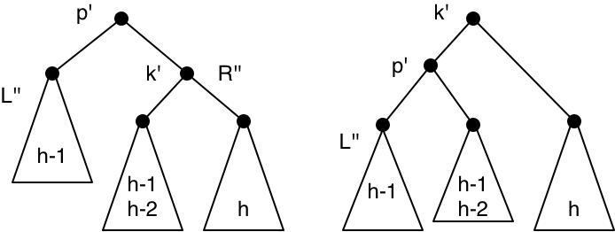
We still have to deal with the third subcase of the second case, which is where \(h(S)=h(R)\). In this case, the height of \(N\) is \(h(L')+1=h(R)+2\), which means there is a violation of the AVL property at \(P'\).
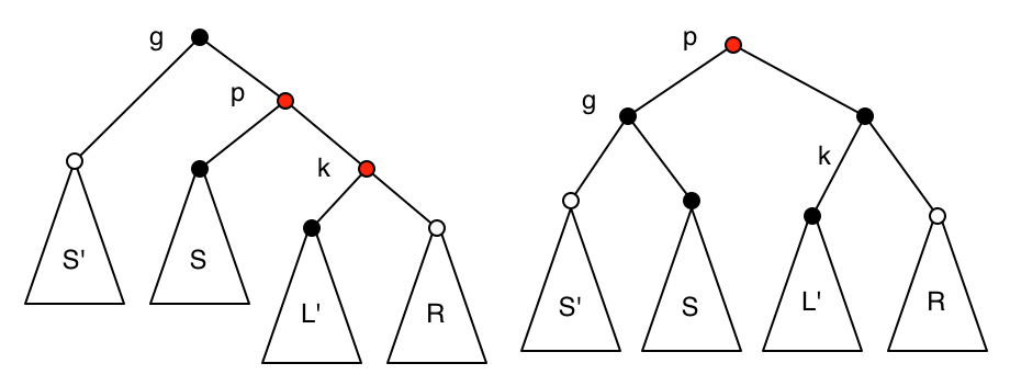
The fix if this happens is shown in the following diagram. It is called a double rotation, because it can be factored into two single rotations (a right rotation at \(k'\), and then a left rotation at \(p'\)). Again, there is a symmetric double rotation for the symmetric situation.
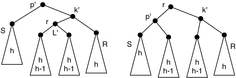
Replacement followed by a double rotation gives a resulting tree where the new parent node has the same height as the parent node of the original. So the height change does not propagate further in the tree.
To summarize the helper function: we head right in \(L\) until we find a right subtree that can be paired with \(R\) in an AVL tree (in the case where \(L\) has greater height). That might cause a double rotation, in which case the work is done, or it might just increase the height when the right subtree is replaced. The increase in height might propagate up the tree and then disappear, or it might require a left single rotation to fix. That might propagate the height increase to the parent, and eventually it might reach the root (in which case the whole tree has grown in height).
The cost of a join on \(L\) and \(R\) is \(O(\max\{h(L), h(R)\})\). If the result has \(n\) nodes, this is \(O(\log n)\). However, this analysis will not let us conclude that split takes logarithmic time. It sufficed for treaps because we could show that the joins done by split were all constant time. But this may not be the case for AVL trees. We need to be more careful about the cost of a join.
The more careful statement, which should be clear from the above discussion is this: The cost of a join on \(L\) and \(R\) is \(O(\max\{|1,h(L) - h(R)|\})\), and the resulting tree either has height \(\max\{h(L), h(R)\}\) or one more than this. This statement will also be true for the remaining two implementations (with a suitable redefinition of \(h\)), allowing us to reuse this analysis later on. For simplicity, we’ll take off the \(O()\) brackets in the cost of a join (instead of carrying along the hidden constant in our calculations).
Now we can analyze split. Recall that this operation splits a tree \(T\) into \(L\) and \(R\) given a key \(k\) (which may or may not be in the tree). It recursively splits the left or right subtree (depending on the comparison of \(k\) and the root key) and then joins the appropriate part of the result with the subtree not recursed upon. We need to bound the work done by the joins. We can show by induction on the height of the tree that the cost is bounded above by \(h(L)+h(R)+h(T)\), and that both \(h(L)\) and \(h(R)\) are bounded by \(h(T)\). This gives us time \(O(\log n)\) to split a tree with \(n\) nodes.
Consider a recursive split on the left subtree \(T_L\). It produces \(L'\) and \(R'\) with cost bounded above by \(h(L')+h(R')+h(T_L)\) and \(h(L')\le h(T_L)\) and \(h(R') \le h(T_L)\) by the inductive hypothesis. The result \(L\) is \(L'\), and the result \(R\) is the join of \(R'\) and \(T_R\), at cost \(O(\max\{|1,h(R') - h(T_R)|\})\).
If the cost of the join is the 1 term in the maximum, then \(h(R')=h(T_R)\), and \(h(R)\) is either the same or one more. Thus the total cost is \(h(L')+h(R')+h(T_L)+1 \le h(L) + h(R)+ h(T)\).
If the cost of the join is \(h(R') - h(T_R)\), then since \(h(R')\le h(T_L)\) by the induction hypothesis, and \(h(T_L)-h(T_R)\le 1\) because this is an AVL tree. So the cost of the join is 1 and \(h(R)\) is either \(h(R')\) or one more. Thus the total cost is \(h(L')+h(R')+h(T_L)+1 \le h(L)+h(R)+h(T)\).
If the cost of the join is \(h(T_R) - h(R')\), then \(h(R)\) is either \(h(T_R)\) or one more. Thus the total cost is \(h(L')+h(R')+h(T_L)+ h(T_R) - h(R')\le h(L)+h(T_R)+h(T_L) \le h(L)+h(R)+h(T)\).
That concludes the inductive step for a left recursion; the right recursion is symmetric, giving us our desired cost bound. This same analysis will work for the next two versions of balanced BSTs, so we have less to cover as we proceed. We can also reuse the analysis of set operations for treaps, which I sketched above, to get worst-case running times of \(O(m \log (\frac{n}{m}+1))\).
A conventional presentation of AVL trees focussing on insert and delete can use the same rebalancing function for both (making use of single and double rotations as we have done here), which is not the case for the next two variations. This, combined with a relatively intuitive balance condition that is easy to reason about, makes it a popular choice for data structures courses.
Even though AVL trees are the oldest variant, and there has been much work since then, they were still chosen to be the implementation for the Map and Set ADTs in the OCaml standard library. In 2014, the team responsible for Core (the proposed alternative standard library used at Jane Street and in the Real World OCaml book) benchmarked all the variants we consider here and some others, and decided to stick with AVL trees. In both OCaml implementations, the height restriction is relaxed so that left and right subtrees can have a height difference of two instead of one. This makes the worst-case depth higher (though still logarithmic), which might make lookups more expensive but simplifies balancing in the other operations. The tradeoff was judged to be worth it.
Exercise 37: Implement join for AVL trees, using the following datatype.
type 'a avl_tree = |
| Empty |
| Node of int * 'a * 'a avl_tree * 'a avl_tree |
|
type 'a bst = 'a avl_tree |
As before, write a is_avl function that runs in linear time. You might wish to use your AVL implementation to do further testing on the derived operations. \(\blacksquare\)
4.1.6 Weight-balanced trees
I will just sketch the ideas in this section, for reasons that will become evident. Weight-balanced trees (WBTs) can be thought of as relaxing the Braun tree condition that the two subtrees have size differing by at most one. Intuitively, think of the weight as the size. The WBT invariant or balance condition is that each subtree has weight no more than \(\delta\) times the weight of its sibling tree, for a fixed constant \(\delta>1\) to be chosen later.
The case of trees of size 2 (with one empty subtree) is awkward; one solution is to take the weight to be the size plus one, and another is to handle an empty subtree as a special case. Both solutions complicate the correctness proof.
The recurrence for the maximum height of a WBT as a function of size resembles \(T(n)=T((1-\frac{1}{\delta})n)+1\), which for \(\delta>1\) has the solution \(T(n)=O(\log n)\).
The balance condition for AVL trees is that the heights of the two subtrees are within 1 of each other. The WBT balance condition is expressed in terms of weight, but if we take logarithms, the logarithms of the weights of the two subtrees are within a constant additive factor of each other.
The code for join for WBTs can be viewed as a variation on the code for height-balanced (AVL) trees. If the two trees \(L,~R\) being joined are in balance, we just use the Node constructor. Otherwise, we recursively descend into the larger subtree. Say it is the left subtree; as with AVL trees, we descend along the right spine until we find a place where the current subtree \(L'\) and \(R\) are in balance. We would like to replace \(L'\) in the result with the tree formed by the join key \(k\), \(L'\), and \(R'\).
But this might violate the balance condition with respect to the sibling of \(L'\). Either a single rotation or a double rotation is necessary at this point, and the algorithm uses another parameter \(\Delta\) to choose. If the replacement has weight more than \(\Delta\) times the weight of the sibling, a double rotation is done, otherwise a single rotation. The imbalance may propagate to the parent and its sibling, so rotations may be needed all the way up the tree.
The code is relatively short and clear, and the analysis goes through as before, if we replace the height of the tree with a measure the original authors call rank, defined as one plus the logarithm of the weight. What remains is the correctness proof, and that is obviously heavily dependent on the choice of the parameters \((\delta,\Delta)\). Whatever the choice, all proofs are lengthy with many cases. But the proof only has to be done once.
The original paper by Nievergelt and Deo (1973) used parameters \((1 + \sqrt{2}, \sqrt{2})\), which is the tightest balance condition that works (and leads to the shortest worst-case trees). But the irrational numbers make for some awkwardness. They have to be approximated in practice, and that could lead to problems in maintaining the balance. It would be better to use rational or even integer parameters.
Adams wrote elegant purely-functional code using WBTs for an ML competition in 1993, but he was more concerned about implementation and benchmarking than correctness proofs. His SML (Standard ML) library (which became the standard) and his implementation for GNU/MIT Scheme (also the standard) used different parameter choices; a port to Data.Map in Haskell used yet another choice. In 2010, a bug report filed for the Haskell library gave an instance involving a deletion from a tree with twelve elements which resulted in an imbalanced tree. It was probably found by randomized testing.
Straka (2010-2012) fixed the Haskell bug by changing the parameters, and produced a careful paper proof of correctness for his choice, as well as benchmarks investigating various choices. Hirai and Yamamoto (2011) found and fixed bugs in the SML and Scheme implementations, characterized the space of possible parameter choices, and produced a formal proof (using Coq) of the correctness of an implementation of the algorithm for proper parameter choices.
Weight-balanced trees provide a good case study of the issues involved in moving from a theoretical design to a widely-used practical implementation.
4.1.7 Red-black trees
Red-black trees are probably the most popular balanced BST implementation, both in terms of actual use and exposure in education. As I mentioned above, they originally developed from work on nonbinary trees where all leaves have the same depth, and are best motivated this way. Without this analogy, the invariant seems mysterious, even though the reasoning is not difficult.
Bayer worked in this setting around 1970, both with small bounds on the number of keys in a node and with large bounds. Trees with large bounds are commonly called B-trees, and are best studied in the context of their major applications, file systems and databases, because low-level aspects play more of a role in their implementation and analysis, and here we are maintaining a high-level fictional view of the machine that ignores virtual memory and caches. Of the trees with small bounds, the 2-3-4 tree is the one we will focus on.
A 3-node contains two keys and has three children.
The left subtree of a 3-node contains keys less than the first root key; the middle subtree contains keys between the first and second root keys; and the right subtree contains keys greater than the second root key.
A 4-node contains three keys and has four children, with the same sort of relationship among keys and children.
Since all leaves are at the same depth and every internal node has at least two children, it is not hard to show that the height of a 2-3-4 tree with \(n\) keys is \(O(\log n)\) (the worst case is a perfect tree). The lookup procedure for 2-3-4 trees is messier than for binary trees, but there are no new ideas, just more cases.
Naive insertion into a binary search tree replaces an empty leaf with a node containing the new key. Insertion into a 2-3-4 tree is similar, but we attempt to insert the key into the parent of the empty leaf. If that would result in four keys in a node, one of the two middle keys is removed, and the node is split into a 2-node and a 3-node (containing the inserted value). But then we continue to insert the removed middle key into the parent. If the top is reached, the key becomes a 2-node.
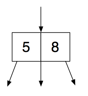
This sounds nice, but actually coding it results in a number of annoying special cases, and deletion is worse. It gets better with an encoding, described by Guibas and Sedgewick, that simulates a 2-3-4 tree by a binary search tree with additional information. In a red-black binary search tree, each node is coloured either red or black. Here is the translation from a 3-node into a black node with a red child.
![]()
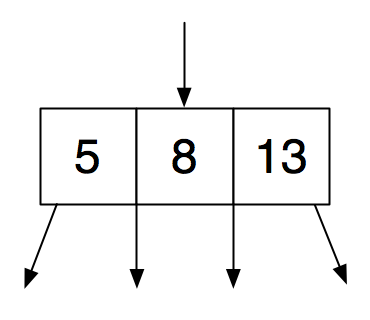
A symmetric translation is also possible, allowing us more flexibility. Here is the translation of a 4-node.
![]()
We see that in such a translation, no red node has a red child. It is also the case that the root is black, but we will relax this requirement, as it is not essential for correctness, and the flexibility helps to extend the previous analysis for union in this framework to this variant.
If we define the black depth of a leaf to be the number of black nodes on the root-leaf path, then all leaves are at the same black depth. But since no root-leaf path has two red nodes in a row, the actual depth of a leaf is at most twice the black depth. This lets us conclude that the height of a red-black tree with \(n\) nodes is \(O(\log n)\).
lookup for a red-black tree is simpler than for a 2-3-4 tree; it simply proceeds as in an uncoloured binary search tree, ignoring colour.
To code join, we define the black height \({\hat h}(T)\) of tree \(T\) to be the maximum black depth of any descendant, and maintain this value at each node in addition to the colour. To join \(L,~k,~R\), we start as with AVL and weight-balanced trees. If the black heights of \(L\) and \(R\) are equal, we apply the Node constructor with these subtrees and \(k\). If the roots of \(L\) and \(R\) are both black, the root of the new tree is red, otherwise it is black.
In the remaining cases, one tree has greater black height. As before, we assume it is \(L\), the other case being symmetric. The recursion proceeds down the right spine of \(L\) until \(L'\) is found with a black root and \({\hat h}(L') = {\hat h}(R)\). We can apply the Node constructor to \(L',k,R\), where \(k\) is coloured red. This result is supposed to replace \(L'\).
But the root of \(R\) could be coloured red, or the parent \(p\) of the replacement could be red. If the parent \(p\) of the replacement is black but the root of \(R\) is red, we recolour the root of \(R\) black and do a single left rotation. This does not change the black depth of any node.

If \(p\) is red, then its parent \(g\) must be black. We recolour \(k\) as black and do a single left rotation. Again, this does not change the black depth of any node.
The rotation results in the new parent being red, so the same logic needs to be used higher up. In other words, when a result is produced by the recursion down the right spine, we are replacing the left subtree recursed upon with the result of the recursion, but if the right child of the result of the recursion is red and its right child is also red, we recolour the second of these two black and do a single left rotation. There is nothing to rotate with when we reach the top, but in this case, if there is a red root with a red right child, we just colour the root black.
The analysis of running time for this variant is like the ones for AVL and weight-balanced trees if, in this case, we define the rank of a red node to be twice its black height minus one, and the rank of a black node to be twice its black height minus two.
A conventional presentation focusses on insertion, and uses both single and double rotations. It also doesn’t maintain the heights of trees, only the colours. Even those can be hidden in unused bits in pointers, in a language like C++ which allows pointer arithmetic. The same thing is true of the information for AVL trees; we just have to maintain the imbalance between sibling trees, and only three values are possible. Finally, the algorithm can be made to operate in a single top-down pass. To get a sense of this, consider insertion into a 2-3-4 tree. If we pass through a 4-node on the way down, we can pre-emptively split it, even if we end up just inserting into a 2-node at the bottom. These should be considered late optimizations, but they dominate some presentations of the material.
Conventional deletion is brutal. It is often left as an exercise, and the exercise is often left undone, even if required of students. Of course, a library implementation must handle it. Our framework avoids the brutality (and even avoids the double rotations that show up in conventional insert code) by refactoring the mess into sequences of splits and joins, reminiscent of how red-black trees avoid the messy details of 2-3-4 trees. It may be worth completing the implementation below simply to be able to boast about it.
There are further refinements possible. Andersson in 1993 created what are usually called AA trees, an encoding of 2-3 trees, which makes for simpler code by removing some cases. Sedgewick rediscovered this idea in 2008 with left-leaning red-black trees, where no red node has a red right child (Andersson’s trees were right-leaning). It is possible to show that red-black trees have constant amortized update cost over a sequence of insert/delete operations starting with an empty tree. This is also true of weight-balanced trees, but not of AVL trees.
Red-black trees are the basis of the Map and Set implementations in the C++ STL and in the Java standard library. However, the recent and increasingly popular languages Scala and Clojure, both of which run on the JVM (Java Virtual Machine), do not use any form of balanced binary trees for their implementations. They use a more recent data structure called HAMT (hash array mapped tries), best learned about after reading the rest of this flânerie. That is also what is used for Racket’s "immutable hash table" data structure.
Exercise 38: Implement join for red-black trees, using the following datatype.
type colour = Red | Black |
|
type 'a rb_tree = |
| Empty |
| Node of colour * 'a * 'a avl_tree * 'a avl_tree |
|
type 'a bst = 'a rb_tree |
As before, write a is_rb_tree function to aid in testing (it should run in linear time).
\(\blacksquare\)
Extended Exercise 39: The simplest non-binary tree is a one-two tree (OTT). It uses a definition like the following:
type 'a ott = |
| Empty |
| One of 'a ott |
| Two of 'a ott * 'a * 'a ott |
An OTT satisfies the BST invariant, namely that the key at a Two node is greater than every key in the left subtree and less than every key in the right subtree. An OTT also satisfies the invariant for nonbinary trees that all Empty leaves will be at the same depth (the height of the tree plus one).
This is not enough to keep an OTT from degenerating to a path, so there is one more invariant: every One node has a Two sibling. As a consequence, the root of an OTT cannot be a One node, and the child of a One node cannot be a One node. Another consequence is that a left or right subtree might not be an OTT (it could be a One node containing a valid OTT).
Your task is to implement insert for OTTs, working out all the details of the algorithm from scratch. As before, you should also consider writing an is_ott function to catch bugs in your code.
To facilitate implementation, we will add to the above datatype definition. Two constructors can be added for temporary use, New and Three. You don’t have to use either or both of them, but using them properly can reduce cases, and can be convenient when dealing with intermediate results which otherwise would have to be put into a tuple or added parameters.
type 'a ott = |
| Empty |
| New of 'a |
| One of 'a ott |
| Two of 'a ott * 'a * 'a ott |
| Three of 'a ott * 'a * 'a ott * 'a * 'a ott |
The idea is that a New node is a temporarily overstuffed Empty node that results from naive insertion. It can be removed right after it is produced as the result of recursive insertion. Similarly, a Three node is a temporarily overstuffed Two node. Removal of a Three node that is produced as the result of recursion might result in the production of a new Three node. Note that no valid OTT contains a New node or a Three node. The insert operation should consume and produce only a valid OTT. New and Three are solely for internal use in the implementation of insert.
Again, the choice is up to you, but consider maintaining an additional invariant on the use of Three: all three subtrees are either Empty or they are Two, One, Two respectively. This might cut down on the number of cases to consider.
State and justify an expression for the smallest number of keys in an OTT of height \(h\), and give an \(O\)-notation bound on \(h\) as a function of \(n\).
Then implement delete, which does not require the use of New or Three.
The unified framework requires binary trees, but it is not hard to adapt the derived operations to the use of One. Another challenge is to implement join for OTTs. My course tutor and I independently worked on this task, and produced different solutions, both more complicated than the other implementations discussed here. Can you come up with an elegant implementation?
The OCaml feature called "polymorphic variants" provides a nice way to avoid completely rewriting the derived functions in the unified framework under circumstances such as this.
OTTs were introduced by Ottmann and Six in 1976, but they came to my attention via a 2009 "functional pearl" paper by Ralf Hinze, to whom I am indebted for details of this exercise. \(\blacksquare\)
4.2 Binary tries
In the previous section, the only computations we did on keys was comparison under some arbitrary total ordering. In this section, we will consider other computations on keys, in order to introduce a data structure that is not only useful for maps, but (suitably generalized) in text processing, as described in the next chapter.
For simplicity, let’s consider the keys to be natural numbers, and once again primarily consider maintaining sets of keys, rather than maps. One powerful computation we can do with a natural number is use it to index an array. If we maintain an array where elements are some representation of "yes" (the index is in the set) and "no" (the index is not in the set), then we can answer membership queries in constant time. Besides the usual problems with arrays, this approach is impractical, as the array has to have size at least \(M\), the size of the largest number in the set.
If you have been exposed to material on computer architecture, you know that memory addresses are treated as sequences of bits to be decomposed by hardware, and the size of memory means that memory accesses are much more expensive than other primitive machine operations. This suggests that we might ourselves consider decomposing keys into sequences of bits, as we did for an index into a sequence in Chapter 2. Let’s start with perfect binary trees with "yes" and "no" stored at the leaves, with navigation on the key in standard binary notation, least significant bit first. Here’s what the tree for the set \(\{1,4,5\}\) would look like. (This set will be our running example.)
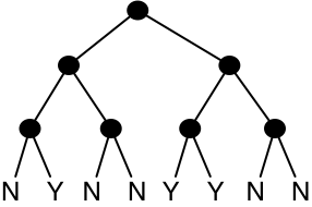
The number of leaves is between \(M\) and \(2M-1\), so the total size of the data structure is still \(O(M)\), and the lookup time is now \(O(\log M)\). We are going to try to preserve the lookup time while reducing the space cost. One obvious optimization is to get rid of trees full of "no". Every subtree with only "no" leaves can be replaced with a single "no" leaf. Here’s what our example set looks like with this optimization.
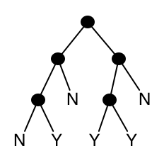
The worst-case lookup time has not changed, but the space requirement has decreased. By how much? For a nonempty set, every "no" is the child of a node whose other child contains at least one "yes". In this fashion, we can associate every "no" with some "yes". How many "no"es can be associated with a given "yes"? At most one for each ancestor of that "yes". So the total space cost is now \(O(n \log M)\), where \(n\) is the number of elements of the set.
The space used by the balanced binary search trees earlier in this chapter was \(O(n)\), so it would be nice if we could achieve that. We no longer have internal nodes all of whose associated leaves are "no". The new worst case is that all leaves are "no" except for one. When doing a lookup, if we reach a subtree with only one "yes" leaf, we can finish things off with a direct equality comparison of the search key and the leaf key. So we replace such a tree with a "yes" leaf containing the key value it represents. For our example set:
We would have to keep a copy of the original key in the lookup, rather than discarding low-order bits as we move down the tree. Alternately, we can store at the "yes" leaf the key value it represents with the appropriate low-order bits removed.
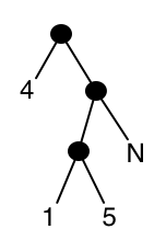
While this can result in some space improvement, the worst-case space cost is the same as before. It’s not hard to construct a tree with \(\Omega(n)\) long paths to "yes" leaves that uses \(\Omega(n \log M)\) space. The final optimization gets rid of those paths, which have many internal nodes with one "no" child. Since we are doing a final equality comparison at a "yes" leaf, we can afford to skip the navigation at these internal nodes even though it might let a failed lookup stop early. We store at each internal node the bit that is used for navigation at that node (represented as a power of 2). Here is the result for our example set.

Now each leaf contains a unique key, so the space cost is \(O(n)\), while lookup is still \(O(\log M)\).
This data structure is called a binary trie. The word "trie" is pronounced like the English word "try", even though it comes from the middle letters of the English word "retrieval", which would suggest a pronunciation like "tree". The basic idea was first proposed in 1959 (for strings, which we will examine in the next chapter), and the final optimization in 1966 by Morrison, with the name "Patricia tree" (sometimes these are called "compressed tries").
The lookup operation has gotten more complicated, so it’s worth summarizing it. The original search key is preserved as we go down the tree. Each internal node is labelled with the bit used for navigation. Arithmetic (or, perhaps, bit operations) can be used to see whether that bit of the search key is 0 or 1, and thus whether to go left or right. Only "yes" leaves remain, and the search key is compared with the leaf key to give the final answer.
What about the other set operations? To facilitate them, we maintain some additional information at the internal nodes, which is the discarded bits that reached that node (as a number). Viewing the bits of a key in standard order, these bits will be a common suffix of the bits of all keys in that subtree. (They are a prefix of the bits viewed in right-to-left order, which is the order in which we view them to navigate.) Lookup could stop early if we check for this common suffix and fail to find it, but this does not change the worst-case running time.
To insert key \(k\) into trie \(t\), we use structural recursion on \(t\). If \(t\) is a "no" leaf, the result is a "yes" leaf containing \(k\). If \(t\) is a "yes" leaf containing \(n\), and \(n=k\), then the new trie is the old trie. If \(n \ne k\), then we need to find the lowest-order bit where they differ and their common suffix. If the numbers are standard 64-bit integers, there are clever ways to use bitwise operations on words to do this in constant time, but it can also be done with the obvious search without changing the asymptotic running time of \(O(\log M)\). In the new trie, the "yes" leaf is replaced by a node with the computed common suffix and bit to navigate on, with children consisting of the old "yes" leaf and a new "yes" leaf containing \(k\).
If \(t\) is an internal node, and \(k\) shares its suffix, then we use its bit to navigate, and recursively insert \(k\) into one of the children. If \(k\) does not share the suffix, we must (as above, so there is scope for shared code here) find a shorter suffix that it does share and bit to branch on, and make a new internal node with this suffix and bit, with one child being \(t\) and the other being a "yes" leaf containing \(k\). All of this pretty much follows from the definition of binary trie.
Inserting into a trie with \(n\) keys takes time \(O(\log M)\), which can be slightly improved to \(O(\min\{n, \log M\})\) if constant-time operations are available to quickly find the lowest different bit of two values. Deletion is left as an exercise for you.
Exercise 40: Implement binary tries, using the following datatype.
type btrie = |
| No |
| Yes of int |
| Node of int * int * btrie * btrie (* suffix, branch bit *) |
|
type intset = btrie |
The two int fields in a Node hold the suffix and branch bit (which is a power of 2) respectively. You should provide the following functions.
val empty : intset |
val lookup : int -> intset -> bool |
val insert : int -> intset -> intset |
val delete : int -> intset -> intset |
As an added challenge, consider implementing set operations. \(\blacksquare\)
Exercise 41: Write a is_binary_trie function that runs in linear time. This is harder than it looks at first. Think carefully about all the relationships among the information contained in a valid binary trie and how you might verify them. \(\blacksquare\)