5 Text Processing

\(\newcommand{\la}{\lambda} \newcommand{\Ga}{\Gamma} \newcommand{\ra}{\rightarrow} \newcommand{\Ra}{\Rightarrow} \newcommand{\La}{\Leftarrow} \newcommand{\tl}{\triangleleft} \newcommand{\ir}[3]{\displaystyle\frac{#2}{#3}~{\textstyle #1}}\)

"Burned all my notebooks / What good are notebooks? / They won’t help me survive"
Talking Heads, "Life During Wartime", Fear of Music, 1979

In our previous treatment of sequences, there was no implied relationship between the elements, apart from the ordering imposed by the sequence. But in many applications, consecutive elements can form larger groupings with relevant meanings. For example, the sequence of characters in a book can be grouped into words, sentences, paragraphs, pages, and chapters. The sequence of nucleotides along a DNA molecule can be considered in a similar fashion, where the groupings may indicate important aspects of biological mechanisms. Text processing has been important from the earliest days of computing (arguably the first stored-program electronic computer was built for just this purpose) but its importance has only increased in recent years. As with many of the topics in this course, the subject is vast, and here I will cover only a small curated selection of classic and recent results.

We will consider text to be stored in a string, a sequence of characters allowing constant time indexing. This suggests an array, but we will consider strings as immutable. We will be using arrays to store information about strings, but we will not be making heavy use of mutation. Many of the algorithms we discuss will write to an array index at most once and only read from that index after a write occurs to it. Or, if there are multiple writes to an array index, all writes take place before all reads. This, like memoization, does not break equational reasoning, and can be considered to be purely functional, with an underlying implementation that uses but does not expose mutation. Arrays in the Haskell programming language (considered to be pure) operate this way.

Most programming languages support a string data type where characters can be stored in a single byte (typically using ASCII encoding). In recent years, the trend has been to make such strings immutable, starting with Java in the mid ’90’s, and continuing with Javascript and Python. OCaml originally had mutable strings, but the language started a gradual shift away from them some years back. While the default compiler setting still works with mutable strings for backward compatibility, new code should avoid mutation, and there is a command-line compiler option to enforce immutability. We will assume that strings are immutable.

String constants look like "this" and have type string. String operations are provided by the String library module (some of which are implemented by algorithms discussed in this module, so be careful which ones you use for exercises!). The expression String.get s i gets the ith character of string s. This can also be written s.[i], and has type char There is a String.set function, but as explained above, you shouldn’t use it (and we won’t need to). The Char library module provides some additional functions for characters. I will mention two here: Char.code consumes a single character and produces a number between 0 and 255 (the eight-bit ASCII encoding interpreted as a natural number), and Char.chr does the opposite. These allow us to pretend that arrays can be indexed by characters, since we can convert a character to the actual numerical index an array requires.

The DNA example above suggests that the flexibility to consider other alphabets may be useful. The main distinction is whether the alphabet is constant-size and known in advance (as with human-language text, and DNA) or unbounded, unknown, and possibly large (say, integers). Some algorithms are sensitive to this distinction (for example, those that might use a character value as an array index, or do other computations on that value), and others are not (for example, if characters are only compared for equality). The first few algorithms we consider will work on arbitrary alphabets, as they only use equality comparisons.

We will use the following mathematical notation in informal descriptions of algorithms: the character at index \(i\) of string \(S\) is \(S[i]\), and \(S[i\dots j]\) represents the substring from indices \(i\) through \(j\) inclusive. The number of characters in \(S\) is the length of \(S\), denoted as \(|S|\). Thus the entire string \(S\) is \(S[0\dots|S|-1]\). (Warning: some books and research papers use 1-based indexing.) A substring of \(S\) starting at index \(0\) is called a prefix of \(S\), and a substring of \(S\) ending at index \(|S|-1\) is called a suffix.

Mathematically, a substring is just a way of focussing attention on a contiguous segment of a string, but computationally, a substring operation (such as the one provided by the String library module) produces a new copy. It is thus not a constant-time operation, and if you use it, you have to take its full cost into account. (It shouldn’t be necessary for any of the exercises here.)

5.1 Simple exact matching

We start with the oldest and simplest problem: given a pattern string \(P\) of length \(n\) and a text string \(T\) of length \(m \ge n\), is the pattern a substring of the text? More precisely, is there an \(i\) such that \(P=T[i\dots i+n-1]\)? Variations include finding the index of the first occurrence, and all occurrences. The term "pattern" suggests a generalization to something other than a string (for instance, allowing "wildcards" that match any character, or more generally, regular expressions) but we will not pursue that tangent here.

There are two classic algorithms for this problem dating from the mid-’70’s, named after their authors: Knuth-Morris-Pratt (KMP) and Boyer-Moore (BM). In the mid-’90’s, Dan Gusfield noticed that a preprocessing step in a paper by Main and Lorentz could be used to give a simpler algorithm, as well as serving as the basis of a unified explanation for these and other algorithms. His description of this simpler algorithm occurs early in his 1997 book, which is a treasure trove of string algorithms (for more details, see the Resources chapter). Gusfield does not give the algorithm a name; I will call it the Gusfield-Main-Lorentz (GML) algorithm.

5.1.1 The naive algorithm

To motivate the preprocessing step in the GML algorithm, let’s consider the naive algorithm, which can be summarized as "try all possible starting points of \(P\) in \(T\)". Conceptually, we align the left ends of pattern and text, and start comparing characters from left to right. When there is a mismatch, we "slide" the pattern forward one character, and repeat the comparison from the left end of the pattern.

More precisely, a single step compares characters \(P[j]\) and \(T[i+j]\) for equality. We start \(i\) and \(j\) at 0, and on a successful comparison, increment \(j\). If \(j\) reaches \(n\), then \(P=T[i\dots i+n-1]\); if this happens, or a comparison is unsuccessful, then \(i\) is incremented and \(j\) starts again at 0. The search terminates when \(i\) reaches \(m-n+1\).

The algorithm can easily be implemented with two nested loops, or with a tail-recursive function. Because the strings are processed from left to right, it can easily be adapted to work with structural recursion on lists of characters. (Many of the algorithms we consider can be adapted for lists of characters.)

Exercise 42: Write OCaml code for the naive exact string matching algorithm. Your function should consume a pattern string and a text string, and produce a list of indices representing positions in the text string where the pattern string appears. The type signature is string -> string -> int list. If you are not used to writing tail-recursive code instead of loops, this is a good opportunity to practice. \(\blacksquare\)

The running time of the naive algorithm is \(O(nm)\). Clearly we must access each character in the pattern and the text at least once, so we cannot hope to do better than \(O(n+m)\). The question is how to achieve this. There are two possibilities to improve the naive algorithm. We could try to slide the pattern more than one position forward based on some information, or we could try to avoid repeating comparisons if we find a mismatch late in the pattern but only slide forward a small amount.

An example of the first possibility occurs if we encounter a character in the text that does not appear in the pattern at all. In this case, we can slide the pattern entirely past that character.

It’s a bit harder to see how to take advantage of the second possibility. The key to understanding it is to notice that a small slide forward means overlap between the old and new positions of the pattern.

If the first character of the new position of the pattern (at index \(0\)) lines up with index \(i\) of the old position of the pattern, and we know that the pattern starting at index \(i\) has a sequence in common with the pattern starting at index \(0\), then we may already know the result of those comparisons with the text.

5.1.2 The Gusfield-Main-Lorentz (GML) algorithm

The observation in the last paragraph of the previous section motivates the following definition of the length of the longest substring of a string \(S\) starting at index \(i > 0\) that matches a prefix of \(S\). \(Z_i(S)\) is the maximum \(j\) such that \(S[0\dots j-1]=S[i\dots i+j-1]\) (or zero if there is no such \(j\)). When \(S\) is clear from context, we omit it and just write \(Z_i\). For \(Z_i>0\), we call the substring \(S[i\dots i+Z_i-1]\) a Z-box.

As an example, suppose \(S\) is aabcaabdaae. \(Z_1\) is 1, as is \(Z_5\) and \(Z_{9}\), but \(Z_4\) is 3 (the associated Z-box is the substring aab starting at index 4) and \(Z_8\) is 2 (the associated Z-box is aa). All other Z-values are zero.

We can compute \(Z_i\) for a given \(i\) by comparing \(S[j]\) with S[i+j] for \(j=0,1,\dots\) until a mismatch occurs or we reach the end of \(S\). Let’s call this a match from scratch at index \(i\). We have to do this to compute \(Z_2\). If we do this for all \(i\), it will take \(O(|S|^2)\) time in the worst case (for example, when \(S\) consists of repetitions of a single character). We can reduce the cost if we use the previous Z-values in the computation.

To this end, we define \(r_i\) for \(i > 0\) to be the rightmost endpoint of the Z-boxes that begin at or before index \(i\). That is, \(r_i\) is the maximum of \(j + Z_j - 1\) over all \(0 < j \le i\) such that \(Z_j > 0\). We also define \(\ell_i\) to be the leftmost endpoint of some Z-box with right endpoint \(r_i\). That is, \(\ell_i\) is the value of \(j\) achieving the maximum.

In our example aabcaabdaae, \(Z_4\) is 3, so \(S[4\dots 6]\) is a Z-box. Consequently, \(r_5\) is 6, and \(\ell_5\) is 4.

Suppose we have computed \(Z_i\) for \(0 < i \le k-1\), and we want to compute \(Z_k\). It turns out that the only \(r_i\) and \(l_i\) values we need are \(r=r_{k-1}\) and \(\ell=\ell_{k-1}\).

If \(k > r\), then there is no previous Z-box reaching index \(k\), meaning that the previously-computed \(Z_i\) values are not going to help us. We compute \(Z_k\) with a match from scratch at index \(k\). If \(Z_k > 0\), then \(\ell_k = k,~r_k = k + Z_k - 1\); if \(Z_k = 0\), then \(\ell_k = \ell_{k-1},~r_k = r_{k-1}\).

This happens in our example aabcaabdaae when computing \(Z_2\), where the match from scratch fails on the first comparison. It also happens when computing \(Z_4\), where the match from scratch fails on the fourth comparison.

But if \(k \le r\), we have some useful information, because index \(k\) is contained in a Z-box, namely \(S[\ell\dots r]\). Call this substring \(\alpha\), and call the part of it starting at index \(k\) (namely \(S[k\dots r]\)) \(\beta\). We’re going to be able to compute \(Z_k\) without doing some comparisons starting from index \(k\), namely those involving characters in \(\beta\).

In our example aabcaabdaae, consider \(5\). At this point, \(\ell=4\) and \(r=6\). \(\alpha\) is aab, and \(\beta\) is ab.

Since \(\alpha\) is a Z-box, \(\alpha = S[0\dots Z_\ell-1]\) and \(\beta = S[k'\dots Z_\ell-1]\) where \(k'=k-\ell\). We make use of the previously computed \(Z_{k'}\).

If \(Z_{k'} < |\beta|\), then we know that a match from scratch at index \(k'\) would do \(Z_{k'}\) comparisons and stop before the end of \(\beta\). So this is also true of a match from scratch at index \(k\), and we don’t have to do any comparisons at all. We can set \(Z_k=Z_{k'},~\ell_k=\ell,~r_k=r\).

This happens in our example aabcaabdaae when \(k=5\), which results in \(k'=1\). Since \(Z_1=1\), we know that a match from scratch at index 5 will have one successful comparison before a failure, and we can avoid doing that comparison.

But if \(Z_{k'} \ge |\beta|\), we know that a match from scratch at index \(k\) would have comparisons succeed at least through \(\beta\). We don’t know whether or not it can go further, so we start a match from scratch at position \(r+1\). If this fails at index \(q\), then \(Z_k=q-k,~\ell_k=k,~r_k=q-1\).

This happens in our example aabcaabdaae when \(k=9\). For another example, consider the string abcabdabcabcd. When \(k=9\), \(\ell=6\) and \(r=10\). \(\alpha\) is abcab, and \(\beta\) is ab, so \(k'=3\). Here \(Z_3=2\), so the next comparison done is between \(S[2]\) and \(S[11]\). That succeeds, but the next comparison fails.

In these examples, \(Z_{k'}=|\beta|\). What if \(Z_{k'} > |\beta|\)? That happens with the string abcabcabcabd, when \(k=9\), \(\ell=6\), and \(r=10\). But in this case the next comparison the algorithm does must fail. Here it is between \(S[2]\) and \(S[11]\). If this was a match, it would mean that \(r\) should be at least 11. This is a possible optimization, but it doesn’t affect the worst-case running time.

That concludes the description of the GML algorithm. There are some clear optimizations: we only need the latest \(\ell,r,k\), and if we start them at \(0\), the \(Z_1\) computation is done as part of the \(r < k\) case. What is its running time? There are \(|S|\) values \(Z_k\) computed, and each one takes time proportional to the number of comparisons done. A comparison either succeeds (match) or fails (mismatch), and there is at most one mismatch for each value of \(k\), so at most \(|S|\) failed comparisons are done. The value \(r\) never decreases; it starts at 0, is incremented by at least the number of successful matches, and cannot reach \(|S|\). So the total time is \(O(|S|)\).

That was just the preprocessing step. We still have to discuss how to use this to do exact matching. It turns out there is a simple way of dealing with the rest of the problem using the computation we have just defined.

Given a pattern \(P\) of length \(n\) and a text \(T\) of length \(m \ge n\), we form the string \(S=P\$T\), where \(\$\) is a character not occurring in \(P\) or \(T\). We then compute the Z-values for \(S\). \(Z_i(S) = n\) for some \(i>n\) if and only if \(S[0\dots n-1] = S[i\dots i+n-1]\), that is, if and only if \(P[0\dots n-1] = T[i-(n+1)\dots i-2]\). So this finds all occurrences of \(P\) in \(T\).

There are some clear optimizations here as well. Since \(\$\) does not occur anywhere else in the pattern or text, all the Z-values are at most \(n\), and \(k'\) defined in the algorithm is at most \(n\). Since we only needed \(Z_{k'}\) for the algorithm, we don’t need to store \(Z_i\) for \(i > n\). We don’t actually need to use \(\$\) or form \(S\), either; that was just a conceptual convenience.

The GML algorithm can be thought of as a preprocessing step where the Z-values are computed for \(P\), followed by a search in the text. Once the pattern has been preprocessed, many different texts may be searched with the same Z-values. It takes time \(O(n+m)\) and extra space \(O(n)\).

The GML algorithm is easier to derive and analyze than the two classical algorithms KMP and BM, mentioned above and described below. Gusfield also showed how to explain those algorithms in an easier fashion using the Z-values. I will sketch these algorithms briefly in the next section; for complete details and discussion, I refer you to Gusfield’s book.

Exercise 43: Write OCaml code for the GML algorithm. The type signature is the same as for the naive algorithm. Besides the space needed for the pattern and text strings and the Z array for the pattern, your code should use \(O(1)\) additional space. This means not explicitly forming the \(P\$T\) string. This complicates the calculation of the Z values for the text string, but with a bit of thought, you should be able to do it in such a way that the core logic can be shared (via a helper function) with the computation on the pattern string. \(\blacksquare\)

5.1.3 An overview of classical algorithms

5.1.3.1 The Knuth-Morris-Pratt (KMP) algorithm

The KMP algorithm (published 1977) was discovered independently by Donald Knuth and Vaughan Pratt at Stanford, and James Morris at CMU. They all wanted to improve the naive algorithm by not "backing up" in the text.

The easiest way to describe the preprocessing of the pattern \(P\) is to define \(sp'_i\) as the length of the longest proper suffix of \(P[0..i]\) that matches a prefix of \(P\), where, in addition, \(P[i+1]\ne P[sp'_i]\). (There is a weaker definition of \(sp_i\) that does not have the additional condition.)

This makes it possible to implement the following "shift rule": when doing a match from scratch at some index, suppose the first mismatch occurs when \(P[i+1]\) is compared with \(T[k]\). Then the pattern is shifted \(i-sp'_i-1\) characters to the right. The definition of \(sp'_i\) guarantees that the first \(sp'_i\) characters of \(P\) in the new position already match the corresponding characters in \(T\), so that the comparison can continue with \(T[k]\) (no backing up). Furthermore, one can further reason that no matches have been missed.

Since the shifting is conceptual, the algorithm is often implemented using a "failure function" \(F'(i)=sp'_{i-1}+1\) and "pointers" (indices) \(t,p\) representing the current point of comparison in \(T,P\) respectively. If \(T[t]=P[p]\), both pointers are incremented. On mismatch, \(p\) is set to \(F'(p)\). If the mismatch occurs at \(p=0\), it remains there and \(t\) is incremented. On a full match, \(p\) is set to \(F'(n)=sp'_{n-1}+1\). (The algorithm is sometimes presented using a finite-state-machine metaphor, but this is unnecessary, and potentially more confusing.)

The \(sp'_i\) definition resembles the definition of Z-values, but it is focussed on the right end of a match with a prefix, instead of the left end. Making the switch is not difficult. To compute the \(sp'_i\), we note that \(sp'_i\) is \(Z_j(P)\), where \(j\) is the smallest value such that \(i = j + Z_j(P) - 1\). We can process the \(Z_j(P)\) for \(j=n-1,n-2,\dots\) and compute the corresponding \(i\), then set a potential value of \(sp'_i\). The last such value written will be the smallest, as required. This takes linear time. (It requires multiple writes to an array, but no reads until after the writes, so it does not break equational reasoning.)

Of course, the original algorithm computed the \(sp'_i\) directly, through reasoning that is similar to what we did for the Z-values, but more complicated. Any conventional presentation of the KMP algorithm will give you a sense of this, or, if you have followed the discussion here closely, you can reconstruct the reasoning yourself. It is also possible to compute the Z-values from the \(sp'_i\) in linear time.

5.1.3.2 The Boyer-Moore (BM) algorithm

The KMP algorithm is often taught in detail, but not used much in practice. In contrast, the BM algorithm (published 1977) is rarely taught in detail, but used a lot in practice. The reasons for not going into detail in a classroom are that the preprocessing is more complicated and the proof of linear time is quite complicated. But the BM algorithm often results in sublinear time matching (this can be shown to hold in expectation under certain assumptions).

The BM algorithm does the match from scratch starting from the right side of the pattern. There are two rules suggesting pattern shifts on mismatch, and the larger of the two is used. The easier rule is called the "bad character" rule. For each character \(x\) that occurs in \(P\), we define \(R(x)\) to be the index of the rightmost occurrence of \(x\) in \(P\) (or zero if it does not occur). The bad character rule says that in a match from scratch, if a mismatch occurs between \(P[i]\) and \(T[k]\), then \(P\) should be shifted right by \(\max\{1,i-R(T[k])\}\) places, in effect to the rightmost place where \(T[k]\) occurs in \(P\) (or past \(k\) if it does not occur).

The more complicated rule is called "the strong good suffix rule", and this is the one that can make use of Z-values. We define \(L'(i)\) to be the largest index \(j < n-1\) such that string \(P[i\dots n-1]\) matches a suffix of \(P[0..j]\) and the character preceding that suffix is not \(P[i-1]\), or 0 if no such \(j\) exists. If a mismatch occurs at \(P[i-1]\) and \(L'(i)>0\), then \(P\) is shifted right \(n-L'(i)\) positions so that \(P[L'(i)]\) is where the right end of \(P\) used to be.

We still have to discuss what happens if \(L'(i)=0\) or if a full match is found, but we can show how to get the \(L'(i)\) values from the Z-values. We define \(N_j\) to be the length of the longest suffix of \(P[0\dots j]\) that is also a suffix of \(P\). It’s not hard to see that \(N_j=Z_{n-j+1}(P^\mathit{rev})\) (where \(P^\mathit{rev}\) is the reverse of \(P\)), and \(L'(i)\) is the largest index \(j < n\) such that \(N_j = n-i+1\). So the \(L'(i)\) can be computed from the Z-values in linear time, using the same idea as for the computation of the \(sp'_i\) in KMP.

To complete the algorithm description, we define \(\ell'(i)\) to be the length of the largest suffix of \(P[i\dots n-1]\) that is also a prefix of \(P\), if one exists, and zero otherwise. We can show that \(\ell'(i)\) is the largest \(j < n-i+1\) such that \(N_j = j\). If there is a mismatch and \(L'(i)=0\), \(P\) is shifted right by \(n-\ell'(i)\) places; if there is a full match, \(P\) is shifted right by \(n-\ell'(2)\) places; and if there is a mismatch at the very start of a match from scratch, then \(P\) is shifted right by one position. That completes the description of Boyer-Moore.

Again, the original publication did not use Z-values, but as with KMP, described the computation of all defined quantities directly using more complicated reasoning. It also did not provide guarantees of running time. The initial proofs (in the KMP paper of 1979) that BM takes linear time, if the pattern does not occur in the text, were quite complicated; nearly fifteen years later, Richard Cole (1991) gave a simpler proof (but still too much to present here) with a better constant. Gusfield’s book contains a complete exposition of this proof.

If the pattern does occur in the text, then the algorithm as presented so far can take \(\Omega(mn)\) time in the worst case, which happens when pattern and text both consist of repetitions of a single character. To fix this, an additional rule, due to Zvi Galil (1979), can be included, in which case worst-case linear time (\(O(m+n)\)) is always achieved. This rule observes that if a shift moves the left end of the pattern past the point where the previous match from scratch stopped, then some prefix of the pattern has already been matched with the text (up to the point where the previous match from scratch started) and so the next match from scratch can stop early.

5.2 Suffix trees

The algorithms of the previous section preprocess a pattern string in time linear in its length, and then use the resulting information to repeatedly match that pattern against various text strings, in time linear in the sum of the lengths of pattern and text. For many situations, the text is large, and that second cost is too high. I argued above that we can’t avoid looking at every character of both pattern and text. But if the text changes only infrequently or not at all (as is the case with, for example, the works of Shakespeare, human-language dictionaries, or genome sequences), then it might make sense to preprocess the text. In these situations, it is the queries or patterns that change more often, and they can be much shorter. The hope is to answer these queries in time that is linear in the pattern length alone.

To satisfy the convention that the variable \(n\) is used to refer to the main size measure of interest, and to match the descriptions in standard references, I will (at the risk of some confusion) switch the roles of \(n\) and \(m\) in this section and the next. The length of the text will be \(n\). The goal is to preprocess the text in \(O(n)\) time and space, and match each new pattern of length \(m\) in time less than \(O(n+m)\). Surprisingly, this can be done, even if there are many matches for a pattern in a large text. All \(k\) matches can be reported in time \(O(m+k)\), if the alphabet is fixed and finite. When \(n\) is much larger than \(m\), this is a clear win.

5.2.1 From suffix tries to suffix trees

The idea is to build a tree where, at a node, a character of a pattern is used as an index into an array of subtrees. This idea resembles the binary tries described at the end of the previous lecture module, but using characters to navigate instead of bits. The trees are thus no longer binary; the number of children of a node can be as many as the number of characters in the alphabet. The other difference is that we used binary tries to represent an arbitrary set of integers, but here we will use a trie to represent a set of strings with a certain relationship: all suffixes of the text string. The resulting structure is called a suffix trie.

As mentioned previously, this technique goes back to the Patricia tree data structure described by Morrison (1968), where "Patricia" is an acronym for "practical algorithm to retrieve information coded in alphanumeric" (it was used for arbitrary sets of strings). I’ll repeat the optimization sequence we went through for binary tries, but quickly, as you’ve already seen it once.

Here is part of the suffix trie for the text mississippi (a commonly chosen example). The white nodes represent points where a suffix ends. Even with this small example, I have to leave out some deep paths (for clarity), such as the one of length 11 containing the whole text. By considering a string with no repeated characters, it should be clear that the space required by this version of a suffix trie is \(O(n^2)\) for a text of length \(n\).

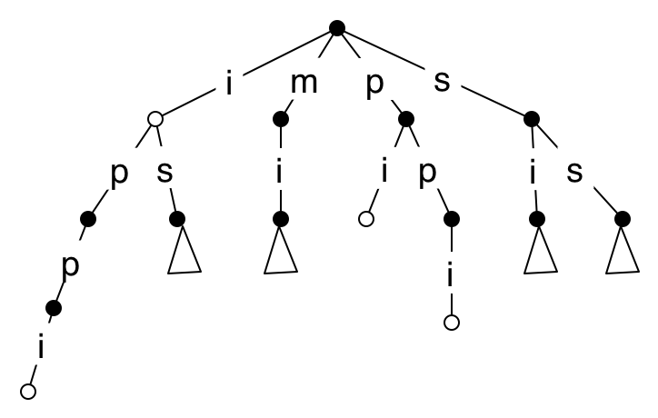
We can now see how to search for a pattern of length \(m\) in \(O(m)\) time, though it’s unclear how to get the index of an occurrence in the text, or the indices of all occurrences. We won’t spend time on that yet, because the space requirements make this method too expensive for long texts, so we need to change the data structure.

A white internal node represents a suffix that is also a prefix of another suffix. We are going to compress the long paths, and these nodes will get in the way. To eliminate them, we can (again, conceptually) add $ at the end of the text, where $ is a character that does not appear in the text. The result is that now all white nodes are at leaves.

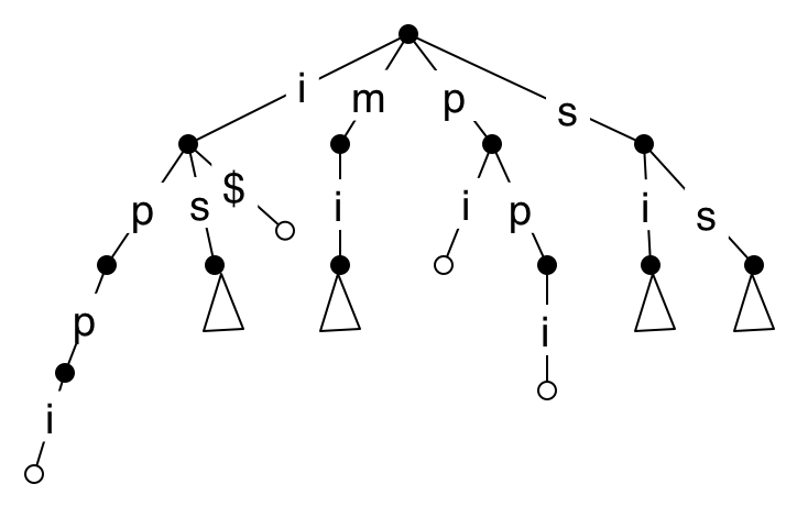
To compress the long paths, we merge each node with a single child with that child. This results in a tree whose internal nodes each have at least two children, and edges are labelled with substrings rather than single characters.

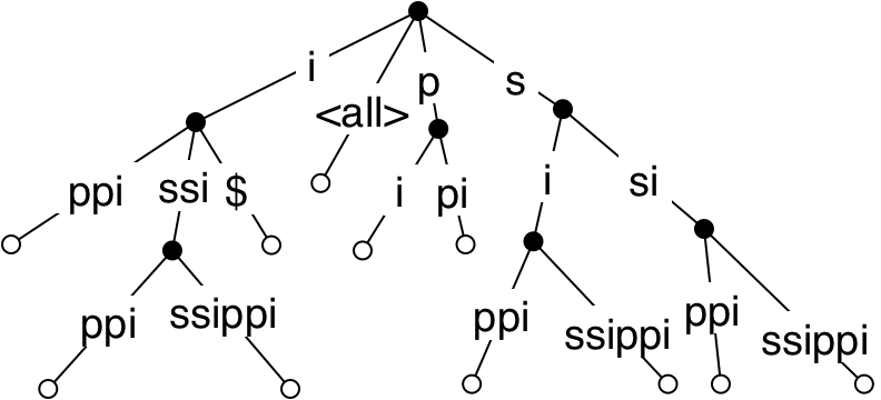
The number of nodes is now \(O(n)\), but the space requirement is still \(O(n^2)\), because each removed node corresponds to an added character in a substring. The final optimization replaces all edge-label substrings, which are just substrings of the text, with the indices of the first and last character in the text. Leaves are labelled with the index in the text of the corresponding suffix. This structure, called a suffix tree, uses \(O(n)\) space.

Lookup of a pattern string uses the characters in order to move down the tree from the root. A full match (after at most \(m\) steps) can happen at a node or in the middle of an edge. In either case, the occurrences of the pattern in the text are given by all leaves in the subtree below. Since each internal node in the tree has at least two children, the number of internal nodes is less than the number of leaves, so if there are \(k\) leaves, they can be collected in \(O(k)\) time by flattening. The total time for the lookup is \(O(m+k)\), as required.

5.2.2 Constructing suffix trees

Given a text string \(T\), the naive approach is to start with a tree with no suffixes (a single node with no children) and then insert the suffixes \(T[i\dots n]\) for \(i=1,2,\ldots n\) one at a time in some order. Naive insertion of a single suffix proceeds as does lookup, using the characters of the suffix in order to move down the tree. A mismatch in the middle of an edge causes the edge to be split and a new node created (which is a leaf if the mismatch occurs on the terminal $, otherwise it is an internal node). One insertion will take time proportional to the length of the suffix, which is \(O(n)\) in the worst case, so inserting all suffixes will take \(O(n^2)\) time.

Exercise 44: Write OCaml code to build a suffix tree from a text string using naive insertion. Use the following datatype, and Char.chr 0 for the $ character.

Then write OCaml code to search for a pattern string in the resulting tree. \(\blacksquare\)

Weiner, who first described the suffix tree data structure in 1973, gave a complicated linear-time algorithm, based on the fact that suffixes share information. It still uses the basic structure of sequential insertion. The approach was improved by McCreight (1976) and Ukkonen (1990), but the resulting algorithms still require a considerable amount of exposition. All three of these algorithms relied on having a constant-sized alphabet. Farach (1997) used a completely different approach to achieve linear time with a polynomial-sized alphabet. His approach recursively computed a suffix tree for indices in odd positions, used that to compute the tree for indices in even positions, and then merged the two. The resulting recurrence looks like \(T(n)=T(n/2)+O(n)\).

Giegerich and Kurtz (1995) investigated functional versions of suffix tree algorithms, and found that a simple lazy algorithm, while having quadratic worst-case time, does well in practice. The idea is to consider all suffixes at once, but leave nodes in the tree unevaluated until a lookup forces them. This will happen naturally when using a lazy language like Haskell, but it can be easily managed in OCaml using the features we have discussed, or even in an imperative language like C++. An unevaluated node conceptually holds a set of suffixes that reached that node (initially there is one node whose set consists of all suffixes). To evaluate such a node during a lookup, the suffixes are grouped by first letter, and each group creates an unevaluated child node, only one of which might be forced by the current lookup. The grouping can be done in time linear in the size of the current set.

Exercise 45: Implement the Giegerich-Kurtz algorithm and test its performance on benchmarks of your own choice. \(\blacksquare\)

Suffix trees use \(O(n)\) space, but the constant can be high in practice, and various methods to reduce the constant can add to the cost of lookup. Lookup is quite fast if the child trees are stored in an array indexed by character. But for the ASCII encoding we are using, this means an array of length 256 at each node, and many array entries will be None (representing empty subtrees). Often this space requirement is unacceptable. How can it be reduced?

If many nodes have few children, the child subtrees can be stored in a list. This list has to be processed sequentially rather than indexed in constant time, meaning a slowdown for search. Other alternatives include using some implementation of Map using balanced trees as in Chapter 4, or hash tables as discussed in Chapter 6.

5.2.3 Applications of suffix trees

There are a large number of applications of suffix trees, particularly in computational biology. A generalized suffix tree handles several texts, by adding text number to leaf tags. This allows, for example, lookup of short DNA sequences in a database of genomes. Suffix trees are also a good starting point for inexact methods, which are important because biological data often contains errors, whether from the sequencing methods or from gene mutation and variation.

A suffix tree for a text can be used to give an efficient implementation of compression as first described by Lempel and Ziv (1977) and widely used (for example, in zip utilities and the GIF standard). We first preprocess the tree by labelling each node \(v\) with the minimum leaf label \(c_v\) in its subtree, which takes \(O(n)\) time.

The idea of compression is to replace a repeated substring in the text at position \(i\) by a pair \((s_i, \ell_i)\), where \(s_i\) is the index of the earlier occurrence of the substring and \(\ell_i\) is its length. To this end, we define \(\mathit{Prior}_i\) to be the longest prefix of \(T[i..n]\) that occurs as a substring of \(T[1..i-1]\), \(\ell_i\) as its length, and \(s_i\) to be its starting index.

Compressing the text is simply a matter of starting \(i\) at 1 and computing \((s_i, \ell_i)\) in a loop. If \(\ell_i>0\), then \((s_i,\ell_i)\) is produced and \(i\) is incremented by \(\ell_i\). Otherwise, \(T[i]\) is produced, and \(i\) is incremented by 1.

For a given \(i\), we find \(\mathit{Prior}_i\) by doing a lookup of the substring of \(T\) starting at index \(i\), until we either run out of text, hit a leaf, there is either a mismatch, or \(i=d+c_v\), where \(d\) is the depth of the search (in characters) and \(v\) is the node we’re at In this last case we have hit the end of \(T[1..i-1]\)), so \(\mathit{Prior}_i\) is \(T[i\dots i+d-1]\); \(s_i\) is \(c_v\), and \(\ell_i\) is \(d\). Since \(i\) is incremented by \(\ell_i\), the total number of comparisons in all searches is \(O(n)\).

The method can be made one-pass by integrating it with one-pass suffix-tree construction (possible with Ukkonnen’s algorithm). As with KMP and BM string searching, this is not the way Lempel-Ziv compression is done in practice, but it provides an easy introduction to the topic, and the actual algorithms can be seen as variations of this basic idea.

Exercise 46: Describe how to use suffix trees to efficiently solve the following problems. If you feel inspired, write OCaml code.

• Give an \(O(|S|)\) algorithm to count the number of distinct substrings that occur one or more times in \(S\).

• Give an \(O(|S|)\) algorithm that, given \(1 \le L \le |S|\), finds the substring of length \(L\) that occurs most often in \(S\).

• Give an \(O(|S|)\) algorithm that finds the shortest unique substring of \(S\), that is, the substring of minimum length that occurs only once.

• Give an \(O(|S|+|T|)\) algorithm to find the longest common substring of \(S\) and \(T\), that is, \((i,j,k)\) such that \(S[i..i+k-1]=T[j..j+k-1]\) and \(k\) is as large as possible.

5.3 Suffix arrays

The idea of suffix arrays was independently introduced by Manber and Myers (1990) in the context of computational biology, and by Gonnet (1987, reported 1992) for a project based at the University of Waterloo involving the Oxford English Dictionary (the genesis of the Open Text corporation). Suffix arrays reduce the high constant on the linear space bound for suffix trees, at some cost for lookups, and can be used for most of the applications of suffix trees. They form a nice case study in techniques that are both interesting and practical.

A suffix array is an array of natural numbers, each one representing a suffix of the text, and the array is sorted by lexicographic order on the suffixes. We illustrate again with the example text mississippi. Here are the suffixes:

And here they are sorted in lexicographic order:

The left column, read from top to bottom, gives the numbers in the suffix array in order. A sorting algorithm can compute the suffix array in \(O(n^2 \log n)\) time (the extra factor of \(n\) is because a single comparison between two different suffixes can take this long). But it is possible to do better, as I’ll discuss below.

Exercise 47: Write OCaml code to compute the suffix array of a string, making use of library sort and string comparison functions. \(\blacksquare\)

5.3.1 Search using a suffix array

Suppose we have a suffix array, and we wish to find a pattern in the text. The search idea is as follows: find the minimum index \(i\) in the suffix array A such that the pattern is a prefix of the suffix starting at \(A[i]\). We can do this using binary search, which you may have seen in your early exposure to computation. If not, the idea is simple. We maintain an interval \([\ell,h]\) within which the target must lie (if it exists), and repeatedly cut it roughly in half. We start with the interval \([0,n-1]\).

One stage of binary search looks at the "middle" element, with index \(d=\lfloor (\ell+h)/2\rfloor\). If the suffix starting at \(A[h]\) is lexicographically equal to the pattern, we have found \(i\). If it is lexicographically greater than the pattern, then the interval is reduced to \([\ell,d-1]\). If is it lexicographically less than the pattern, the interval is reduced to \([d+1,h]\). Since the interval is cut at least in half at each stage, \(O(\log n)\) stages suffice. The suffix-pattern comparison can be naively performed in \(O(m)\) time, so the computation of \(i\) takes \(O(m \log n)\) time. A similar binary search can find the maximum index \(j\) with the same property.

Every suffix in the suffix array between indices \(i\) and \(j\) inclusive is an occurrence of the pattern, and there can be no other occurrences. Thus all \(k\) occurrences can be reported in \(O(k + m \log n)\) time. (The additive \(k\) can be dropped if the implicit representation of the answer in terms of \(i\) and \(j\) is good enough.) But we can do better than this.

Exercise 48: Write OCaml code that consumes a text string and produces a search function that consumes a pattern string and uses binary search on the suffix array to report all occurrences. \(\blacksquare\)

The idea to improve the running time of search is to maintain, along with the interval \([\ell,h]\), the length \(p_\ell\) of the longest common prefix of the pattern and the suffix starting at \(A[\ell]\), and the length \(p_h\) of the longest common prefix of the pattern and the suffix starting at \(A[h]\). The smaller of these represents the length of the longest common prefix of the pattern and all suffixes indicated by entries in the suffix array in the interval \([\ell,h]\). This means that the suffix starting at \(A[d]\) and the pattern have at least this many initial characters in common, and the comparison can start after that point. (This should remind you of the saving in the computation of Z-values earlier, though there is no direct connection, just a similar approach.)

Exercise 49: Adapt your solution to the previous exercise to incorporate the improvement just described. \(\blacksquare\)

The worst-case running time is still \(O(k + m \log n)\), but in practice (as reported by Manber and Myers) this speeds up the algorithm as much as the next idea, which improves the worst-case time to \(O(k + m + \log n)\). I will sketch this idea, because it is a lovely algorithm, and it eventually leads to a way to use suffix arrays in place of most applications of suffix trees.

The idea is to precompute longest common prefix values for all possible bound positions that the binary searches might use. This is a bit tricky because we don’t know the pattern and have to use only the text. For a stage of the binary search as described above, we have indices \(\ell,d,h\). What we will use is the length \(p_{\ell,m}\) of the longest common prefix of the suffix starting at \(A[\ell]\) and the suffix starting at \(A[m]\), and length \(p_{m,h}\) of the longest common prefix of the suffix starting at \(A[m]\) and the suffix starting at \(A[h]\). We will also continue to maintain \(p_\ell\) and \(p_h\) as described above.

Assuming we can look up the precomputed new quantities in constant time, how do we use them? If \(p_\ell = p_h\), we simply continue the string comparison from the next character, as above. If \(p_\ell > p_h\), we consider three subcases depending on the relationship of \(p_{\ell,m}\) and \(p_\ell\).

If \(p_{\ell,m} > p_\ell\), then the suffixes in the array from indices \(\ell\) to \(m\) share a common prefix that is longer than the one that the suffix at index \(\ell\) shares with the pattern. Thus the pattern cannot be a prefix of any of these suffixes, and no further comparisons are needed to reduce the interval to \([m+1,h]\). Similarly, if \(p_{\ell,m} < p_\ell\), then the pattern cannot be a prefix of any of the suffixes in the array from indices \(m\) to \(h\), and no further comparisons are needed to reduce the interval to \([\ell,m-1]\). In the third subcase, \(p_{\ell,m} = p_\ell\), and we can continue the string comparison from the next character.

The remaining case, \(p_\ell < p_h\), is symmetric, with three subcases depending on the relationship of \(p_{m,h}\) and \(p_h\). The key to the analysis is that the maximum of \(p_\ell\) and \(p_h\) never decreases, and if \(k\) characters are examined in a stage, then that maximum increases by \(k-1\). If we split this into \(k\) and \(1\), then the sum of the \(k\)’s is at most \(m\), and the sum of the \(1\)’s is \(O(\log n)\) (the number of stages).

This precomputation can be done in \(O(n)\) time (an interesting algorithm in its own right), and reduces the cost of a comparison in the binary search to \(O(1)\) (since we know that the characters right after the common prefix must be different), so the worst-case running time for lookup is now \(O(m + \log n)\).

How do we compute all the \(p_{\ell,m}\) and \(p_{m,h}\) we need? First of all, how many such quantities are there? Conceptually, form a tree of intervals, with \([0,n-1]\) at the root, and give each node \([\ell,h]\) children \([\ell,m-1]\) and \([m+1,h]\), as long as these intervals are of length at least two. This is a binary tree with leaves of the form \([i,i+1]\), and there are \(n-1\) of them. So there are \(O(n)\) nodes.

There is one computation for the leaves and another for internal nodes. For the leaves, we have to compute, for every \(k \in [0,n-1]\), the longest common prefix of the suffix starting at \(A[k]\) and the suffix starting at \(A[k+1]\). An array indexed by \(k\) containing these quantities is called the LCP array by many references, and is useful in other situations.

Manber and Myers showed how to compute the LCP array along with the suffix array (I will describe the latter below). But Kasai et al. (2001) gave an elegant linear-time algorithm to compute the LCP array from the suffix array. They start by observing that the suffix array is a permutation of the integers in \([0,n-1]\), and so the inverse permutation (which maps \(k \in [0,n-1]\) to the location in the suffix array containing the value \(k\)) can be computed in linear time. We can define the successor of \(k\) to be the value in the suffix array at index one higher than the index where \(k\) is stored (or the suffix starting at this position). Clearly, the successor can be computed in constant time, given the inverse permutation.

Exercise 50: Write OCaml code to compute the inverse permutation of a permutation. \(\blacksquare\)

Now consider the longest common prefix of the suffix starting at index 0 (that is, the whole string) and the successor of 0 in the suffix array. This can be computed by matching starting at the beginning of each string. Suppose the value computed is \(k\) (comparison \(k+1\) failed). The key observation is that the longest common prefix of the suffix starting at index 1 and the successor of 1 in the array is at least \(k-1\). This is true because the suffix starting at index 1 is just the suffix starting at index 0 with the first character removed. So the suffix starting at index 1 shares a prefix of length \(k-1\) with the successor of 0 with its first character removed. The successor of 1 has at least this common prefix with the suffix starting at index 1, and maybe more. We start the character comparisons after this prefix.

The reasoning holds not just for 0 and 1 but for any \(i\) and \(i+1\). An analysis similar to the one we did for the binary search above gives linear time for the whole computation.

This allows us to return to our conceptual tree of intervals and assign to each leaf \([i,i+1]\) the value in the LCP array at index \(i\). Now consider an internal node \([\ell,h]\). The key observation is that the quantity we wish to associate with this node, namely the length of the longest common prefix of the suffix starting at \(A[\ell]\) and the suffix starting at \(A[h]\), is the minimum of the quantities associated with the children of this node. That makes the rest of the LCP computations particularly simple. We don’t need to store the results in a tree; the \(m\) associated with an interval \([\ell,h]\) can’t be associated with any other interval, so we can use an array indexed by \(m\).

Exercise 51: Prove the observation in the paragraph above. \(\blacksquare\)

That concludes the description of how to precompute the quantities needed to speed up the binary search in the suffix array. Here we only needed the length of the least common prefix for specific pairs of suffixes. The ability to compute this for any pair of suffixes is of use in certain string algorithms. This is possible with further preprocessing of the LCP array to allow range minimum queries (another interesting problem in its own right, but one I will leave you to look up).

5.3.2 Constructing a suffix array

Given a suffix tree, we can obtain the suffix array in linear time using structural recursion where edges out of a node are searched in lexicographic order. Since linear-time suffix tree construction algorithms exist (though I have not described any here), this means that linear-time suffix array construction algorithms exist. But this is not very satisfying.

We can do a bit better than naive sorting by adapting the Giegerich-Kurtz top-down approach for suffix tree construction. The idea is to start with an unsorted array containing integers representing all suffixes, and then group elements by the first character of the suffix. This provides enough information to move each array element to an appropriate location in constant time. The grouping takes \(O(n)\) time, after which the algorithm recursively works on each group, ignoring the first character of each suffix.

If all suffixes repeatedly fall into one group (for example, the string consists of repetitions of a single character), this gives \(O(n^2)\) worst-case time. But if groups are reasonably balanced, the algorithm does better than this in practice, just as was the case for the suffix tree construction.

We can view this simple algorithm as first sorting the suffixes by prefixes of one character, then two, then three, and so on. The original Manber-Myers paper on suffix arrays instead doubled the length of the prefix at each pass. Suppose the array is sorted by prefix of size \(k\), and we know the current inverse permutation and the boundaries of each group with a common prefix of that size. What the next pass needs to do, to result in the array being sorted by prefix of size \(2k\), is to sort each group with a common prefix of size \(k\) by their next \(k\) characters, which is the same as taking off the common prefix and sorting by the next \(k\) characters. But since the whole array is sorted by prefix of size \(k\), and taking off the common prefix just results in another suffix, the information needed is already present in the array.

The idea that completes a pass in linear time goes like this. Consider the first suffix in the first group. Suppose it starts at \(A[i]\). What do we know about the suffix starting at \(A[i-k]\)? It has to go into the first subgroup of its group, because if you remove its first \(k\) characters, the resulting suffix (namely the one starting at \(A[i]\)) is in the first group. So we put it there, and then continue by considering the second suffix in the first group, and so on. The accounting details to keep track of where we next fill in each subgroup of each group are a little involved; you can try to work them out for yourself if the idea intrigues you, or look them up in the paper. Since each pass takes \(O(n)\) time, and there are \(O(\log n)\) passes, the algorithm takes \(O(n \log n)\) time.

Several \(O(n)\) algorithms have been developed subsequently, of which the most elegant is due to Kärkkäinen and Sanders (2003). In a manner similar to what Farach’s algorithm does for suffix trees, their algorithm recursively computes the suffix array at two-thirds of the indices (those not congruent to 0 mod 3), computes a suffix array for the remaining indices from that, and then merges the two. The algorithm is simpler and easier to understand than any of the optimal suffix tree algorithms, and the code is relatively compact. Subsequent improvements (as recent as 2015) have concentrated on improving the constants in the linear time bound, and reducing the working space requirements, at the cost of complicating the algorithm somewhat.

Kasai et al., in their paper showing the elegant LCP array construction algorithm, also showed how to use suffix arrays plus LCP arrays to simulate algorithms using bottom-up structural recursion on suffix trees. Follow-up work by Abouelhoda, Kurtz, and Ohlebusch (2004) broadened the class of suffix tree algorithms that can be simulated by suffix arrays together with additional computed information, including bringing the cost of search down to \(O(m)\).

Exercise 52: The following theorem characterizes the suffix array of a string.

Using this characterization, describe how to test whether an array \(A\) is the suffix array of \(S\) in \(O(|S|)\) time. \(\blacksquare\)

Exercise 53: Prove the theorem above. (This idea is due to Burkhardt and Kärkkäinen, from 2003.) \(\blacksquare\)