8 Trees
\(\newcommand{\la}{\lambda} \newcommand{\Ga}{\Gamma} \newcommand{\ra}{\rightarrow} \newcommand{\Ra}{\Rightarrow} \newcommand{\La}{\Leftarrow} \newcommand{\tl}{\triangleleft} \newcommand{\ir}[3]{\displaystyle\frac{#2}{#3}~{\textstyle #1}}\)
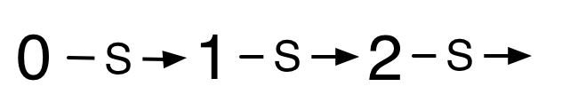
Our unary representation of Nats was inefficient because we only had a choice of a single data constructor. This conceptual diagram from the previous chapter showed the relationships between different natural numbers in terms of the relationships between their representations.
By using two data constructors instead of one, we could do better.
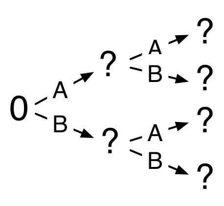
Using two data constructors allowed us to create small representations of many different natural numbers. We’ll adapt this idea to create a data structure holding many different values that lets each of them be accessed more efficiently.
8.1 From lists to trees
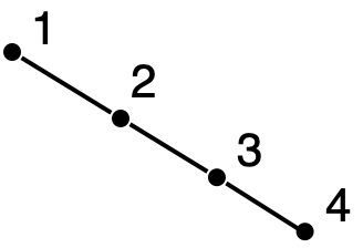
A list exhibits a linear structure similar to our conceptual diagram of our unary representation of Nats.
(cons 'A (cons 'B (cons 'C (cons 'D empty))))
extend consumed an element \(e\) and a sequence \(S\) and produced the new sequence \(e,S\).
head consumed a non-empty sequence \(S\) and produced the element \(e\), where \(S = e,S'\).
tail consumed a non-empty sequence \(S\) and produced the sequence \(S'\), where \(S = e,S'\).
For Racket lists, the implementations of these operations are cons, first, and rest. We now add a new operation, index, which consumes a natural number \(i\) and a sequence \(S\) and produces the \(i^{th}\) element of \(S\) (counting from zero). We say this element has index \(i\) in \(S\). \(S\) must have length greater than \(i\).
Here is an implementation for Racket lists.
| (define (list-ref i lst) |
| (cond |
| [(empty? lst) (error "no element of that index")] |
| [(zero? i) (first lst)] |
| [else (list-ref (sub1 i) (rest lst))])) |
For example, (list-ref 2 '(A B C D)) is 'C.
list-ref is a predefined function in Racket. Our code for list-ref does structural recursion on the natural-number index and the list representing the sequence. The total number of recursive applications of list-ref is the minimum of the index and the length of the list. Can we do better than this?
Our goal is to create a representation of sequences that supports the four operations (extend, head, tail, index) but improves the running time for index. We’ll take as a starting point our development of S-lists from lecture module 05, which we quickly abandoned in favour of Racket’s built-in list representation.
| (define-struct Empty ()) |
| (define-struct Cons (fst rst)) |
Data definition: an S-list is either a (make-Empty) or it is (make-Cons v slist), where v is a Racket value and slist is an S-list.
The linear structure of S-lists results from having a single field (rst) in the main constructor that contains an S-list (another instance of the same datatype). To allow easier access to more data, we add a second such field. Here is the result, with a new set of names.
| (define-struct Empty ()) |
| (define-struct Node (val left right)) |
Data definition: a binary tree is either a (make-Empty) or it is (make-Node v lft rgt), where v is a Racket value and lft and rgt are binary trees.
Here are a few small examples.
make-Empty
(make-Node 14 (make-Empty) (make-Empty))
| (make-Node 6 |
| (make-Empty) |
| (make-Node 14 (make-Empty) (make-Empty))) |
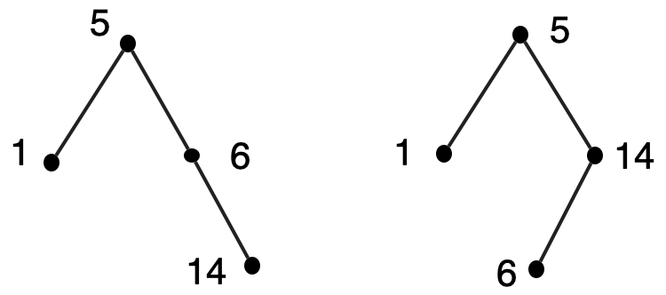
| (make-Node 1 |
| (make-Node 5 (make-Empty) (make-Empty)) |
| (make-Node 6 |
| (make-Empty) |
| (make-Node 14 (make-Empty) (make-Empty)))) |
Trees are heavily used in computer science. The term "tree" is obviously a botanical metaphor, and some of the terminology we use to talk about trees comes from botany. But some of it comes from the idea of family trees. Unlike both physical trees and family trees, trees in computer science are usually drawn branching downward.
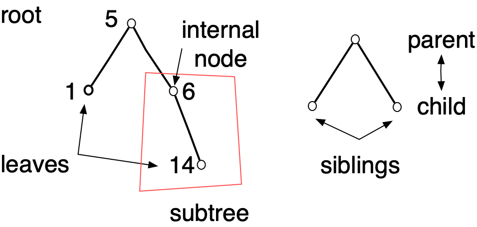
A Node structure satisfying the definition of a binary tree is said to be the root of that tree. Any Node structure it contains is an internal node which defines a subtree. Leaves are Node structures whose left and right fields hold Empty structures, as with the nodes whose value is 14 in the above examples. If a Node structure has Node structures in its left and right fields, those two Node structures are siblings, and children of the enclosing Node structure. We can also use terms like grandparent, grandchild, ancestor, and descendant.
We’ll start our work with binary trees with a very specific construction to solve our sequence indexing problem.
8.2 Braun trees
In our binary representation of natural numbers, we had one constructor, Z, to represent zero, and two constructors, A and B, to form nonzero-even and odd numbers respectively.
We’ll do something similar in placing elements of a sequence into a binary tree, but with the indices of the elements. The element of index zero will be in the val field of the root of the tree, the elements of odd index will be in the left subtree, and the elements of nonzero-even index will be in the right subtree.
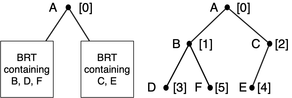
As an example, let’s consider representing the sequence A,B,C,D,E,F. Since the element of index zero is stored in the root, our representation will be (make-Node 'A ... ...). We have to fill in the ellipses.
We will distribute the rest of the sequence among the left and right subtrees of the root. The elements whose indices are odd numbers will go in the left subtree. These are B, D, F. The elements whose indices are even numbers (but not zero) will go in the right subtree. These are C, E. We will store them in the subtree in the order in which they appear in the odd- or even-indexed subsequence, recursively. That is: the left and right subtrees will also be Braun trees. Continuing the process, we get the following.
| (make-Node 'A |
| (make-Node 'B |
| (make-Node 'D (make-Empty) (make-Empty)) |
| (make-Node 'F (make-Empty) (make-Empty))) |
| (make-Node 'C |
| (make-Node 'E (make-Empty) (make-Empty)) |
| (make-Empty))) |
The numbers in square brackets are the sequence indices. Here’s a larger example, with the square brackets and values removed for clarity.
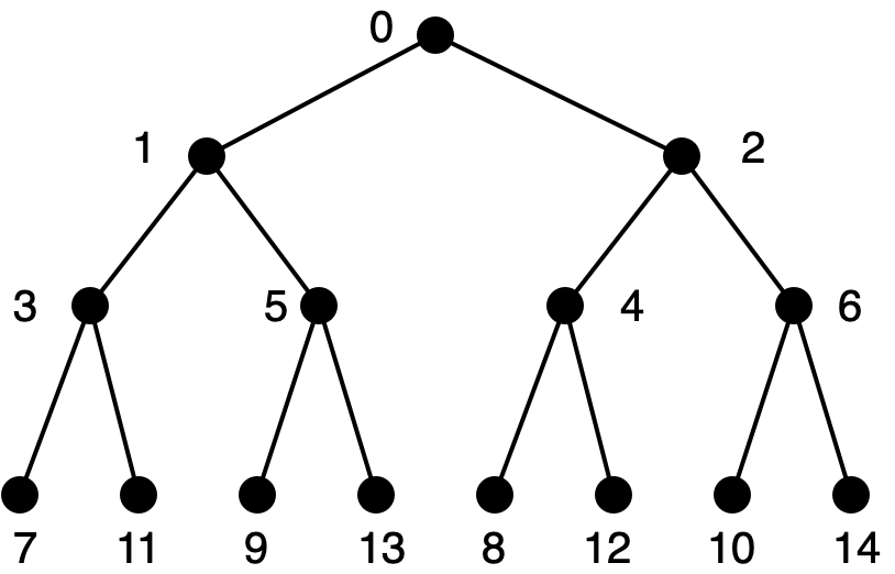
How do we find the element of index \(i\)?
| (define (brt-ref i brt) |
| (cond |
| [(Empty? brt) (error "index too large")] |
| [(zero? i) (Node-val brt)] |
| [(odd? i) (brt-ref ... (Node-left brt))] |
| [(even? i) (brt-ref ... (Node-right brt))])) |
We must compute, from the index of the desired element in the whole sequence, its index in the odd-index or even-index subsequences that are stored in the left or right subtree respectively. Here is the left subtree shown twice. On the left side, it has indices when considered as the left subtree of the whole Braun tree. On the right side, it has indices when considered as a separate Braun tree in its own right.
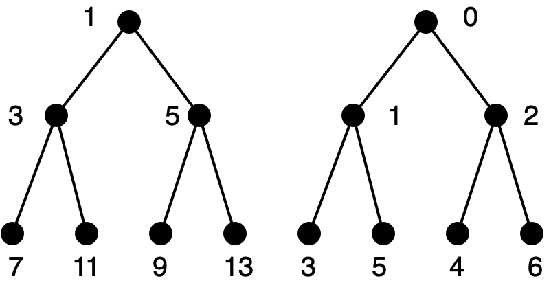
The element at index \(i\) in the whole sequence (for odd \(i\)) is found at index \((i-1)/2\) in the odd-indexed sequence (stored in the left subtree). Here is the right subtree, displayed as above.
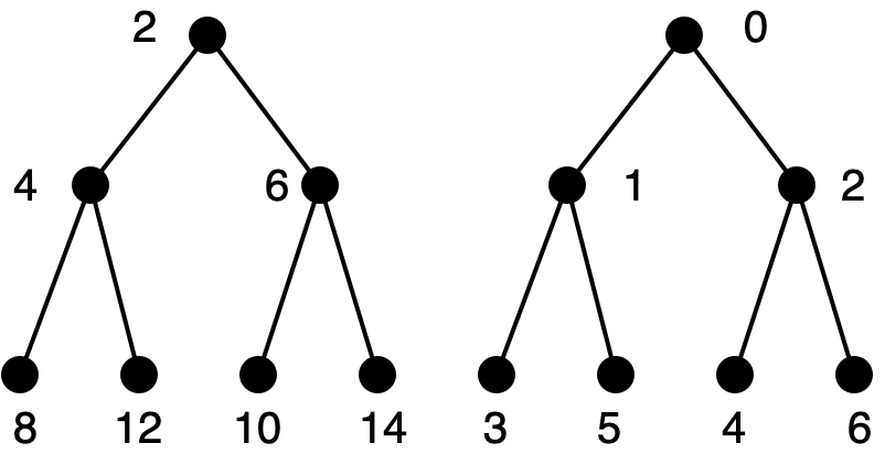
The element at index \(i\) in the whole sequence (for nonzero even \(i\)) is found at index \((i/2)-1\) in the even-indexed sequence (stored in the right subtree).
| (define (brt-ref i brt) |
| (cond |
| [(Empty? brt) (error "index too large")] |
| [(zero? i) (Node-val brt)] |
| [(odd? i) (brt-ref (/ (sub1 i) 2) (Node-left brt))] |
| [(even? i) (brt-ref (sub1 (/ i 2)) (Node-right brt))])) |
Intuitively, this looks like it will be more efficient than lists. Let’s try to quantify that. Let \(T_1(i)\) be the number of applications of brt-ref on a Braun tree and a valid index i.
\begin{align*}T_1(0) &= 1\\ T_1(2k+1) &= 1 + T_1(k)\\ T_1(2k+2) &= 1 + T_1(k)\end{align*}
To get a sense of how this function behaves, we can tabulate the first few values.
\(n~~~\) |
| \(T_1(n)\) |
\(0\) |
| \(1\) |
\(1\) |
| \(2\) |
\(2\) |
| \(2\) |
\(3\) |
| \(3\) |
\(4\) |
| \(3\) |
\(5\) |
| \(3\) |
\(6\) |
| \(3\) |
\(7\) |
| \(4\) |
This is enough for us to figure out a plausible characterization.
Conjecture: For \(2^k \le i+1 < 2^{k+1}\), \(T_1(n)=k+1\).
Another way of saying this:
For \(k \le \log_2 (i+1) < k+1\), \(T_1(n)=i+1\).
Or: For \(i\ge 0\), \(T_1(i)=\lfloor\log_2 (i+1)\rfloor +1\).
These conjectures can be proved by mathematical induction, and confirm logarithmic running time for this case.
Let \(T_2(n)\) be the number of applications of brt-ref on a Braun tree representing a sequence of length \(n\) and an invalid index.
\begin{align*}T_2(0) &= 1\\ T_2(2k+1) &= 1 + T_2(k)\\ T_2(2k+2) &= 1 + T_2(k)\end{align*}
Clearly \(T_2(n)=T_1(n)\). We conclude that the number of applications of brt-ref on a Braun tree representing a sequence of length \(n\) and an index \(i\) is \(\lfloor\log_2 (\min\{i+1,n+1\})\rfloor +1\).
Another way of looking at the running time on an invalid index is to note that each recursive application of brt-ref is done on only one subtree. We define the height of a Braun tree to be the maximum number of applications of Node-left or Node-right before reaching (make-Empty). The total number of applications of brt-ref on a Braun tree is bounded above by the height plus 1. A Braun tree of size \(n\) has height at most \(\lfloor\log_2 n+1\rfloor\).
Reasoning about height works because the recursion is done on only one subtree. For a task where recursion may be performed on both subtrees (for example, an "element-of" operation), the number of recursive applications can be as big as the size.
We have been focussing on the index operation, and Braun trees perform quite well, but perhaps the other sequence operations are much harder on a Braun tree. As you probably guessed, this is not the case. The head operation is implemented by Node-val and so takes constant time. We can ensure running times for implementations of extend and tail that are comparable to the running time of index, that is, roughly logarithmic in the length of the sequence. This is not as good as with lists (where these operations take constant time) but it is still pretty good.
The key is to ensure that recursion is done on at most one subtree. Suppose we are trying to extend A,B,C,D,E,F with Q, which goes at the front of the new sequence. Clearly Q is at the root of the new tree. Everything in the old sequence has index one greater in the new sequence. That means the old odd-indexed sequence is the new even-indexed subsequence. In other words, the new right subtree is the old left subtree, unchanged, so no further computation need be done on it.
What is the new odd-indexed subsequence? It is the old even-indexed subsequence with the former root value A extending it. This is a recursive application on the old right subtree. But we need do only one recursive application, so the efficiency is comparable to brt-index with an invalid index.
Similar reasoning works for the tail operation and for other useful operations. You should work out the details.
Exercise 38: Write brt-extend (consuming a Braun tree and a new element, and producing a Braun tree) and brt-tail (consuming a Braun tree, and producing a Braun tree). brt-tail should raise an error containing "empty" if it is applied to an empty Braun tree. The efficiency of these operations should be logarithmic in the number of elements.
Then write brt-update, which consumes a Braun tree t, an index i, and an element elt, and produces the Braun tree representing the sequence that t represents, except that the element of index i is elt. The efficiency of brt-update should be the same as brt-index, and brt-update should signal an error if the index is out of range. All your code should use structural recursion on Braun trees. \(\blacksquare\)
Exercise 39: Write a function that verifies whether a Racket value is a Braun tree. Note that the number of nodes in a Braun tree uniquely determines its shape.
The goal is to ensure that the efficiency of your solution is roughly proportional to the size of the tree, and not larger than this. To reach this goal, you must ensure that you do at most one recursive application on each subtree. Furthermore, you are going to need more information from the recursive application than simply whether or not the subtree is a valid Braun tree. To this end, the specification of the main function you will write is a little unusual.
You will write the function brt-verify, which consumes a Racket value t and produces false if t is not a valid Braun tree. If t is a valid Braun tree, brt-verify will produce some useful non-Boolean value. You get to choose this value in order to facilitate your implementation. Choosing wisely will make your job easier. Spend some time thinking before you start coding.
Given an implementation of brt-verify meeting this specification, it is easy to write a verification predicate (one that always produces a Boolean value), as shown below.
| (define (valid-brt? t) |
| (cond |
| [(boolean? (brt-verify t)) false] |
| [else true])) |
In full Racket, any non-false value passes a conditional test, not just true. So there would be no need for the additional code of valid-brt?. \(\blacksquare\)
Exercise 40: The illustration of a Braun tree annotated with the indices of nodes is reminiscent of the diagrams (brancing to the right) that we used to figure out binary notation in the Efficient Representations chapter.
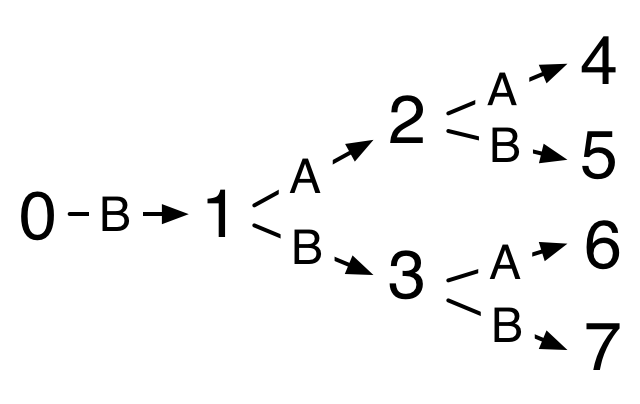
This suggests an alternate binary representation for natural numbers that avoids the awkwardness of rules like "Don’t apply A to Z". Using two alternate constructors C and D, we can add one when taking a left branch and the other taking the right branch, where the number being represented is the index of the node reached in a large enough Braun tree. No additional rules are needed to ensure unique representation.
Write a data definition for this alternate binary representation, and write efficient code for addition and multiplication. \(\blacksquare\)
Braun trees are a specific type of binary tree that allow us to store a sequence in a manner that permits logarithmic-time index operations. We have sped up indexing relative to the list implementation, but for lists, the extend and tail operations take constant time, while they take logarithmic time for Braun trees. There is a more clever (and more complicated) data structure that achieves constant time for extend and tail, while maintaining logarithmic time for index.
Braun trees are an excellent introduction to the study of trees, but they are not used much in practice. Instead, more general data structures that implement "finite maps" are used. Braun trees have logarithmic height, but for some purposes, it is difficult to make use of them, and the shape requirements must be relaxed to gain needed flexibility. This topic is treated in greater detail in my flânerie Functional Data Structures (FDS).
8.3 Tree-structured data
With Braun trees, we took a mathematical concept (sequences) that had no inherent tree structure, and imposed structure on it to improve efficiency. Many forms of data already have structure that lends itself naturally to a tree representation. A book may be divided into chapters, each chapter may be divided into sections and subsections, which contain paragraphs and words. Web pages are specified in a language (HTML) which is tree-structured. In fact, most languages created for processing by computers (programming or specification) are best handled by treating uses as trees. We will take a look at one line of development for which Racket is well-suited, thanks to its list abbreviations.
Consider a Racket expression using only numbers, and addition and multiplication with two arguments.
We can represent this by a variation on binary trees. The val field in a Node structure can hold the operation, and the left and right fields can hold the operands. The Empty structure is replaced by a number. While this works, we can also use lists, which are made more convenient for this purpose because of quote notation.
'(* (+ 3 4) (+ 1 6))
(list '* (list '+ 3 4) (list '+ 1 6))
Data definition: a binary arithmetic S-expression (BAS-exp) is either a number or a (list op lft rgt), where op is either '+ or '*, and lft and rgt are BAS-exps.
The term "S-expression" is used for tree-structured data formed using list constructors. Here we add the adjectives "binary arithmetic" to specify a restricted version. As before, the data definition leads to a template for writing functions that consume BAS-exps. For clarity, we define synonyms for list accessor functions that we use to retrieve components of an expression.
| (define op first) |
| (define left second) |
| (define right third) |
| (define (my-base-fn base) |
| (cond |
| [(number? base) ...] |
| [(list? base) ... (op base) ... |
| ... (my-base fn (left base)) ... |
| ... (my-base-fn (right base)) ...])) |
Using the above template, it is not hard to write an evaluator. Anticipating future expansion, we use a helper function to perform operations.
| (define (eval base) |
| (cond |
| [(number? base) base] |
| [(list? base) (apply (op base) |
| (eval (left base)) |
| (eval (right base)))])) |
| (define (apply op val1 val2) |
| (cond |
| [(symbol=? op '+) (+ val1 val2)] |
| [(symbol=? op '*) (* val1 val2)])) |
We can generalize our representation of arithmetic expressions to operations with more than two operands. We can also allow symbols as well as numbers, letting us represent algebraic expressions with variables. If we add binding forms such as let, function creation like lambda, and conditionals like cond, we will have an interpreter for a Racket-like language written in Racket. Doing some of this work ourselves provides insight into factors that influenced the design of Racket and its tools, and lets us experiment with alternate syntax and semantics. We’ll do this in more detail in a later chapter.
8.4 Binary search trees
When we used ordered lists to improve the efficiency of set operations in the Lists chapter, they had a dramatic effect on the efficiency of intersection and union, but not as much on the element-of operation. Can we use trees to improve efficiency?
We can try. We’ll put the elements of the set in the val fields of binary tree nodes, and impose ordering restrictions on the tree, as we did for ordered lists. The restriction will be that all the elements in the left subtree of the root will be less than the one at the root, all the elements in the right subtree of the root will be greater than the one at the root, and the left and right subtrees will themselves satisfy these restrictions. This is known as a binary search tree. The representation is not unique.
It’s not hard to write code for the element-of (or "search") operation that uses structural recursion on only one subtree. For example, when searching for the element 10 in the above trees, there’s no need to look at the left subtree of the root, since that will contain only numbers less than 5.
Exercise 41: Write the element-of function for a set of numbers represented by a binary search tree. It consumes a number and a binary search tree, and produces #true exactly when the number is in the set. Then write the add function, which consumes a number and a binary search tree, and produces a binary search tree with the number added to the set of elements of the tree (without duplication if it is already there). For an extra challenge, write a remove function (this is messier, and may require helper functions). \(\blacksquare\)
Exercise 42: Write the Racket function valid-bst? which produces true exactly when its argument is a valid binary search tree. Your function should run in time roughly proportional to the number of nodes in the tree. I suggest the same approach as taken in exercise 39 above. \(\blacksquare\)
Structural recursion on only one subtree will guarantee running time roughly proportional to the height of the tree. If the set is known in advance and static, we can build a tree that is suitably short and "bushy", like a Braun tree. But the add function in the previous exercise suggests one might want to maintain sets dynamically during the course of a computation. Your answer to the exercise probably doesn’t guarantee that trees will always be "short". It’s not obvious how to do this efficiently, even for static sets. In the worst case, every left subtree is empty, and the tree is no better than an ordered list.
The solution (or perhaps I should say "solutions", because there are many of them) involves "rebalancing" the tree with local reorganizations during an add or remove operation, to preserve the property that the binary search tree has height roughly proportional to the logarithm of the number of elements. Unfortunately, these solutions are too complicated to present here. I describe a general framework for implementation and analysis in my flânerie Functional Data Structures (FDS).
Simple implementations of binary search trees still make for good programming exercises, and they will come up again in the next chapter.