9 Generative Recursion
\(\newcommand{\la}{\lambda} \newcommand{\Ga}{\Gamma} \newcommand{\ra}{\rightarrow} \newcommand{\Ra}{\Rightarrow} \newcommand{\La}{\Leftarrow} \newcommand{\tl}{\triangleleft} \newcommand{\ir}[3]{\displaystyle\frac{#2}{#3}~{\textstyle #1}}\)
I have been emphasizing the use of structural recursion where possible, but sometimes it is too restrictive. As stated earlier, a function is generatively recursive if the recursive applications in its body do not depend solely on the form of the data it consumes, but are "generated" by computation involving the specific value consumed. It is the most general form of recursion, and it is necessary in many instances. The difficulty with generative recursion is that arguing about or proving correctness and termination gets harder, as typically does the analysis of running time.
Consider a function that uses structural recursion on a list parameter. Termination follows because in the recursive application, the list argument is structurally smaller, and eventually the empty case is reached. Correcteness can often be proved by structural induction, the generalization of mathematical induction to recursively-defined datatypes. For lists, this means coming up with a logical statement describing correctness, showing that it holds when the list parameter is empty, and then showing that if the statement holds when the list parameter is lst, then it holds when the list parameter is (cons v lst) for any v.
As a concrete example, we can consider a function to sum up a list of numbers.
| (define (sum-lists lst) |
| (cond |
| [(empty? lst) 0] |
| [else (+ (first lst) (sum-lists (rest lst)))])) |
How might we prove this correct? The problem is that if you want a precise definition of "sum up a list of numbers", I can’t think of a better one than this code. But we can prove various properties of this function by structural induction. For example, for all lists of numbers lst1 and lst2, (sum-lists (append lst1 lst2)) equals (+ (sum-lists lst1) (sum-lists lst2)). This can be proved by structural induction on lst1.
I have been being vague about these arguments, often omitting them, just as I have been being vague about efficiency. I have two other flâneries that get more precise. Functional Data Structures (FDS) gets more precise about efficiency without neglecting correctness, and Logic and Computation Intertwined (LACI) gets more precise about correctness without neglecting efficiency. Section 1.6 of LACI shows how to complete the proof I alluded to in the previous paragraph (for a closely-related statement). Here I will continue to just sketch ideas, in preparation for that.
To see what happens when we violate structural recursion, let’s do it just a little bit. Here is another function to sum up a list of numbers.
| (define (sum-helper lst n) |
| (cond |
| [(empty? lst) n] |
| [else (sum-helper (rest lst) (+ n (first lst)))])) |
| (define (sum-lists2 lst) |
| (sum-helper lst 0)) |
sum-helper does not use pure structural recursion, because of the way the second argument of the recursive application is constructed. This is sometimes called structural recursion with an accumulator, because the second argument is accumulating information about the list (in this case, a partial sum). Termination is still obvious, since that argument only involves the first (list) argument.
But what about correctness? Since I argued that sum-lists was the best definition of summing a list of numbers, we would need to show something like "For all lists of numbers lst, (sum-lists2 lst) is equal to (sum-lists lst)". This is equivalent to showing "For all lists of numbers lst, (sum-helper lst 0) is equal to (sum-lists lst)".
However, a direct proof of this using structural induction will not go through. You can take my word for it, or you can try doing it yourself. If you try it yourself, you will probably be able to come up with a more clever and complicated statement which implies the original statement, and which can be proved by structural induction.
The further we get from structural recursion, the more complicated our proofs will get. This extends to the kinds of informal reasoning we do when we write code that violates structural recursion. It often gets harder to reason about efficiency as well. In this chapter, I’ll illustrate this phenomenon with a few examples.
9.1 Greatest common divisor
The greatest common divisor (GCD) of two natural numbers \(n\) and \(m\) is the largest natural number that exactly divides both of them. We denote this by \(\mathit{gcd}(n,m)\), and define \(\mathit{gcd}(0,0)\) to be \(0\). (It’s usually defined for integers, and the algorithm we’ll come up with will work for all integers, but it’s just simpler to not have to think about negative number cases, and to think about structural recursion on natural numbers.)
It’s not hard to come up with a structurally recursive algorithm. Try every number from the minimum of \(n\) and \(m\) down towards zero and see if it exactly divides both \(n\) and \(m\). Stop as soon as you find one. For integer division, we’ve already seen Racket’s predefined quotient function; the related function we need is remainder. But this is not very efficient. As previously discussed, integer division is efficient because the underlying machine uses a binary representation; it takes time roughly logarithmic in the value of the dividend. But the number of divisors tried could be large, if \(n\) and \(m\) are different prime numbers (whose GCD is 1).
What we’ll do is replace the larger of the two numbers by something "smaller", such that the new pair has the same GCD. If \(d\) divides \(n\) and \(m\), then it divides any integer linear combination of them, that is, it divides \(an+bm\) for any integers \(a,b\). Suppose \(n > m\). Then \(n - m, m\) has the same GCD as \(n,m\), and we have made the problem "smaller".
If \(n - m > m\), we can repeat the subtraction, and get \(n-2m, n-3m, \ldots, n-qm\) where \(0 \le n-qm < m\). \(q\) is the quotient and \(r=n-qm\) the remainder when \(n\) is divided by \(m\). These are what Racket’s quotient and remainder functions compute, so we might as well use remainder instead of repeated subtraction. We jump from the pair \(n,m\) to \(m,r\). If \(m > n\), this just swaps the two, after which the earlier analysis holds.
When does this process stop? When one of the numbers is zero, the other is the GCD of the original pair. (This takes care of the missing case above, when \(m = n\), because the remainder is zero.) Here’s the code.
| (define (gcd n m) |
| (cond |
| [(zero? n) m] |
| [(zero? m) n] |
| [else (gcd m (remainder n m))])) |
This process is known as "Euclid’s algorithm", and appears in the classic geometry textbook Elements by the 3rd-century BCE Greek author. It is one of the earliest documented algorithms. Edna St. Vincent Millay may have poetically declared, "Euclid alone has looked on Beauty bare", but this process was probably known to the earlier Pythagorian school, and has been independently discovered by other cultures (notably Chinese and Indian).
gcd is a predefined function in Racket. This code definitely uses generative recursion. How efficient is it? After the first recursion (which might just switch the arguments), the second argument goes down by at least one for each recursive application. But this very simple analysis doesn’t show the code to be any better than the structurally-recursive solution, when in practice it seems much faster.
(gcd 20220401 19181111)
\(\Rightarrow^*\) (gcd 20220401 19181111)
\(\Rightarrow^*\) (gcd 19181111 1039290)
\(\Rightarrow^*\) (gcd 1039290 473891)
\(\Rightarrow^*\) (gcd 473891 91508)
\(\Rightarrow^*\) (gcd 91508 16351)
\(\Rightarrow^*\) (gcd 16351 9753)
\(\Rightarrow^*\) (gcd 9753 6598)
\(\Rightarrow^*\) (gcd 6598 3155)
\(\Rightarrow^*\) (gcd 3155 288)
\(\Rightarrow^*\) (gcd 288 275)
\(\Rightarrow^*\) (gcd 275 13)
\(\Rightarrow^*\) (gcd 13 2)
\(\Rightarrow^*\) (gcd 2 1)
\(\Rightarrow^*\) (gcd 1 0)
\(\Rightarrow^*\) 1
To improve the analysis, let’s think about how we can slow the algorithm down, in order to construct a bad case. If \(n\) is much larger than \(m\), then the remainder on division is much smaller than \(n\), which feels like a lot of progress. We use the remainder computation to replace repeated subtraction, but if \(m\) is close to \(n\), the remainder computation only replaces one subtraction, not many. If this is the case, then the pair \(n,m\) is replaced by the pair \(m,n-m\). Another way of saying this is that the pair \(m+k,m\) is replaced by the pair \(m,k\). We can run this process backwards and get a series of growing pairs such that, when viewed forwards, each remainder operation is just one subtraction. If we start the backwards run with the pair \(1,0\), we get \(2,1\), then \(3,2\), then \(5,3\)...
These will be familiar to you if you did Exercise 37 in the Efficient Representations chapter. They are consecutive Fibonacci numbers. In that exercise, the Fibonacci numbers were defined as by \(f_0 = 0\), \(f_1 = 1\), \(f_i = f_{i-1} + f_{i-2}\) for \(i > 1\), and the closed-form solution was given as \(f_i = (\phi^i - (1-\phi)^i)/\sqrt{5}\), where \(\phi = (1+\sqrt{5})/2\). Our construction suggests the following claim.
Claim: Applying gcd to \(f_{i+1}\) and \(f_{i}\) results in \(i\) applications of gcd in total.
The claim can easily be proved by mathematical induction on \(i\). Since the closed-form solution indicates that Fibonacci numbers grow exponentially with their index, we can conclude that the number of recursive applications is roughly proportional to the logarithm of the second argument for this series of examples.
We’ve constructed a series of bad examples (well, modestly bad) but how do we know that these are the worst cases? Intuitively, any deviation from the remainder operation being a single subtraction only helps the algorithm go faster (which, viewing the process backwards again, makes the pairs grow quicker). The following claim makes this concrete.
Claim: If (gcd n m) requires \(i\) applications of gcd for \(n>m\), then \(n \ge f_{i+1}\) and \(m \ge f_i\).
Again, this can be proved fairly easily by mathematical induction on \(i\). This shows that consecutive Fibonacci pairs are the worst case, and we conclude that the running time of gcd is roughly proportional to the logarithm of its smaller argument.
This section demonstrates some common issues with generative recursion. First, the need to discuss termination, usually by showing that some function of the arguments is decreasing with each recursion but is also bounded from below. Second, the need to provide often complex and ad-hoc arguments to establish the running time.
An interesting application of the Euclidean algorithm was demonstrated by Eric Bjorklund when considering the distribution of timing pulses for components of the SNS particle accelerator at the Oak Ridge National Laboratory in the US. A given number of pulses needed to be distributed into a fixed number of slots (that repeat cyclically, like hours on a clock) so that they were spread out as evenly as possible. This is obvious if the number of slots is a multiple of the number of pulses. For twelve slots and four pulses, they go in slots 1, 4, 7, and 10, and there are two empty slots between each pulse. We could represent this as [100100100100].
But for thirteen slots and five pulses, the answer is not so obvious (you might be able to come up with one, but we are looking for a general algorithm). The result will have five filled slots and eight empty slots. Bjorklund suggests initially viewing this as and [0][0][0][0][0][0][0][0] and [1][1][1][1][1]. Each of these two groups, viewed separately, is an optimal distribution: zero pulses over eight slots, and five pulses over five slots. Distributing the [1] sequences among the [0] sequences gives [01][01][01][01][01] with [0][0][0] left over. Again, each of these, separately, is an optimal distribution: five pulses over ten slots, and zero pulses over three slots. Distributing the [0] sequences among the [01] sequences gives [010][010][010] with [01][01] left over. The next distribution gives [01001][01001] with [010] left over. There is only a single leftover sequence now, and it doesn’t matter where it goes (because the pattern repeats cyclically), so we can just put it at the end. The final arrangement is [0100101001010].
Looking at the numbers of sequences in our two groups, we start with (8,5), then (5,3), (3,2), and (2,1). These are the numbers we would get from a GCD computation, which makes sense, as the number of leftovers is the remainder from integer division. Computationally, we shouldn’t take the above representation too literally; there are clearly only two different sequences at any point, each of which is repeated multiple times (first [0] and [1], next [01] and [0], and so on). We can just maintain the two sequences and the number of repetitions of each.
Exercise 43: Write a Racket function that consumes the total number of slots and the number of pulses, and produces a list of 0’s and 1’s representing an optimal distribution. Your code should run in time roughly proportional to the number of slots, though you might want to work through the rest of this chapter first to get more experience, if you want to ensure this and be able to justify it. \(\blacksquare\)
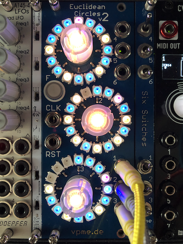
Godfried Toussaint observed that many of these distributions correspond to complex rhythms from music around the world. Subsequently, the algorithm has been implemented in various programs and devices for use in electronic music. Here is some hardware I own for this purpose (with the capability to quickly alter the number of slots, number of pulses, and start position).
9.2 Sorting
Sorting is frequently discussed in introductions to computer science, because its specification is easy to understand, and it admits many different algorithms. These features make it a good source of examples in this chapter. We have already used ordered lists when implementing set operations, but here, duplicate values are permitted, so we speak of the lists as being in non-decreasing order. Once again, we’ll assume that list elements are numbers. It is easy to generalize each algorithm to arbitrary elements with a comparison function provided as an additional argument.
9.2.1 Insertion and selection sort
Unlike with GCD, structural recursion can be used to implement sorting, and this provides a nice contrast with later examples. If we recursively sort the rest of the argument list, we are left with the problem of inserting the first of the argument list into the resulting sorted list. The insertion helper function can also use structural recursion. This is very similar to Exercise 21 in the Lists chapter, and is known as insertion sort.
Exercise 44: Write Racket code for insertion sort. \(\blacksquare\)
What is the efficiency of insertion sort? The insertion helper function can take time proportional to the length of its argument, and it is applied once for each element in the list to be sorted. So the running time is roughly proportional to the square of the number of elements.
Jeremy Gibbons, in a paper titled "How To Design Co-Programs", points out that many uses of generative recursion can be understood by reference to the concept of structural co-recursion. Structural recursion does a case analysis on the argument; structural co-recursion does a case analysis on the result. For lists, this involves answering the following three questions:
When is the result empty?
What is the first of a non-empty result?
What is the argument to the recursive application which computes the rest of a non-empty result?
For sorting, the answers are:
When the argument is empty;
The smallest element of the argument list;
The original argument list with one instance of the smallest element removed.
This is known as selection sort, because we select the element to go first before doing recursion on what remains. It is structurally co-recursive.
Exercise 45: Write Racket code for selection sort. \(\blacksquare\)
Selection sort also takes time roughly proportional to the square of the number of elements. But in practice, insertion sort is preferable. Insertion sort can be faster on already-sorted or near-sorted data, as the insertion helper function can often end its recursion early. But selection sort is not adaptive in this fashion. Nonetheless, it is a good introduction to the idea of co-recursion, which we can use to make the ideas behind many generatively recursive functions less ad-hoc.
9.2.2 Treesort
We saw that binary search trees could be used to add structure to a set for the purpose of answering element-of queries. We can also use them in a sorting algorithm. The idea is to insert the elements of the argument list into a binary search tree, and then "flatten" the tree to a sorted list.
Insertion of a single element into a binary search tree can be done by structural recursion on the tree. Inserting of all elements in the argument list to be sorted can be done by structural recursion with an accumulator (the tree being built). Finally, flattening can be done by structural recursion on the tree. The sorted lists that result from recursion on the left and right subtrees can be put together with the root element (between them in value) using append.
Exercise 46: Write Racket code for treesort. \(\blacksquare\)
We were disappointed in our hopes that binary search trees could improve the efficiency of set operations without more sophisticated code for rebalancing, and we will be similarly disappointed here. If the argument list is already sorted, the tree to be built will look like the bad case in the Trees chapter (essentially a list slanting down to the right). In this case, treesort acts like insertion sort, and takes time roughly proportional to the square of the number of elements.
Exercise 47: Flattening using pure structural recursion takes time roughly proportional to the square of the number of elements in the worst case, just by itself. (Can you specify the worst case?) By adding an accumulator, the time can be reduced to roughly proportional to the number of elements. The accumulator will hold a list to be appended to the final result. Complete the code and the justification. \(\blacksquare\)
9.2.3 Quicksort
Gibbons observes that we can implement the building of the binary search tree in treesort by using structural co-recursion on the tree.
Exercise 48: Write Racket code for this second version of treesort, using structural co-recursion to build the binary search tree. To implement the answer to the third question of the recipe for structural co-recursion, you may find the filter function useful. \(\blacksquare\)
The tree built is the same as the earlier version, even though the code looks different and the building is done in a different order. This second version lets us remove the trees entirely from the algorithm. The structural co-recursion in the build function generates argument lists for the recursive applications that will build the left and right subtrees. Instead of building those trees and then flattening them, we can recursively sort those lists. This algorithm was named Quicksort by its inventor, Tony Hoare, and dates from 1959.
Exercise 49: Write Racket code for Quicksort. \(\blacksquare\)
Despite its name, Quicksort isn’t faster in gross terms, as it has the same worst case argument and running time (to within a constant factor) as treesort. We need a different idea to crack the "square of the number of elements" barrier.
9.2.4 Bottom-up mergesort
Mergesort, as its name implies, is based on a function that merges two sorted lists (of arbitrary length) into a single sorted list. The merge function is similar to the union set operation on ordered lists from the Trees chapter.
Exercise 50: Write Racket code for the merge function. \(\blacksquare\)
The running time of the merge function is roughly proportional to the total number of elements in the result. We will look at two different ways of using it to do sorting. The first approach is "bottom-up" (the reason for the name will eventually be clear). It uses three helper functions. The first helper function takes the list to be sorted and puts each element into its own list. That is, the result of applying this helper function is a list of one-element lists. Notice that a one-element list is trivially sorted.
The second helper function takes a nonempty list of sorted lists and merges them in pairs. If there are four sublists, the first two are merged, and the last two are merged. If there is an odd number of sublists, the last one is left as is, since it has no partner. This function can be written using structural co-recursion.
The third helper function repeatedly applies the second one until the result list contains only a single sorted list. This is generative recursion, but of a fairly simple nature.
Finally, the mergesort function applies the first helper function to the list to be sorted, then applies the third helper function to that, and produces the first (and only) element of the result. No recursion is used here, and the empty list is a special case.
Exercise 51: Write Racket code for bottom-up mergesort. \(\blacksquare\)
This version of mergesort is more rarely presented, but I chose to show it first because it is easier to analyze its running time. The first helper function takes time roughly proportional to the number of elements. In the second helper function, each sublist is involved in one merge, so we add up the times for those, and get time roughly proportional to the number of elements. But the second helper function is applied repeatedly, so we have to multiply this time by the number of applications.
How many times is the second helper function applied? The first time it is applied, it is applied to a list of one-element lists. The result is a list of two-element lists, except possibly for the last sublist (which might be a one-element list, if the total number of elements is odd). These two things remain true with each application except the last one: the result is a number of lists of the same length, except for the last list which might be shorter, and the length of the first sublist doubles with each application. The last application might be on a list containing two sublists, the second shorter than the first.
Since the length of the first sublist is growing exponentially with the number of applications, the number of applications is at most logarithmic in the number of elements. Thus the total running time is roughly proportional to the product of the number of elements and the logarithm. If there are \(n\) elements to be sorted, the running time is roughly proportional to \(n \log n\), an improvement over \(n^2\) for the previous sorting algorithms.
9.2.5 Top-down mergesort
The code for top-down mergesort is more direct. There are two special cases, when the argument list is empty or when it contains one element. Otherwise the argument list is split in equal halves (or almost-equal if the number of elements is odd), the two halves are recursively sorted, and then they are merged.
Exercise 52: Write Racket code for top-down mergesort. Your code to generate the halves should run in time proportional to the total number of elements. \(\blacksquare\)
The analysis is easy when the number of elements \(n\) is a power of two, say \(n = 2^k\). The odd case never happens, and all the merges of lists of size \(2^i\) take time roughly proportional to \(n\), for \(i=0,1,\ldots, k-1\). Thus the total running time is proportional to \(k2^k\) or \(n \log n\). Unfortunately, the odd cases make things messier. They can be handled by elementary means, but it’s tedious, and the result is the same in the end. Most presentations wave their hands about the details. I won’t go further here, but my flânerie Functional Data Structures provides you with the ingredients and recipe. Hint: the magic phrase is "Akra-Bazzi"...
Gibbons, in the paper mentioned above, shows how top-down mergesort can be viewed as we did with treesort and Quicksort, except with a different intermediate tree representation that moves values in internal nodes down to leaves, a structurally co-recursive building of the tree from the input list, and a structurally-recursive production of the sorted list from the tree using merges.
This concludes our look at generative recursion as a subject of focussed study. We will continue to use it, as well as the other forms of recursion, in the final chapter of this part of the flânerie.