Example 6.3: BesselY near z=0
Consider again ](images/TPapprox_353.gif) , the Bessel function of the second kind as in Example 6.1, and consider the series expansion first for the case when the order
, the Bessel function of the second kind as in Example 6.1, and consider the series expansion first for the case when the order  is a non-integer.


 |
(6.3.1) |
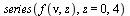
In general for any order  , the expansion about
  starts with a term in
  .
.

 |
(6.3.2) |
Fact: For any order  ,
,  as
as  .
.
In the overall approximation scheme for this function, evaluation at points  where
where  is close to
  will be handled by summing the series expansion.
For our general bivariate approximation scheme based on tensor product series, we will restrict the region away from  . In other words, the restriction is
  where, for example, we may choose
  .
.
Still, polynomial approximation requires a high degree due to the nearby singularity.


 |
(6.3.3) |

 |
(6.3.4) |

 |
(6.3.5) |


 |
(6.3.6) |
The  command has computed the "infinite" Chebyshev series, truncated where the magnitude of the terms becomes smaller than the specified precision
  . Thus the degree obtained is a measure of the "approximation degree" required for the given function.
Multiplication by  yields a function which is finite at
  .
.
 |
(6.3.7) |
 |
(6.3.8) |


 |
(6.3.9) |
This achieves some reduction in the degree required for polynomial approximation.
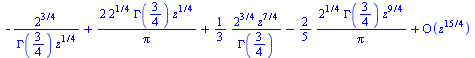
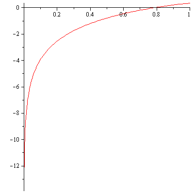
However, the series expansion reveals a square root singularity at  . For the case of integer order
  , the series expansion reveals a logarithmic singularity at
  . In both cases, rational approximation will be advantageous.
Trying various rational degrees  decreasing from degree
  , we find that degree
  is sufficient to achieve the desired accuracy
  .
.
![`assign`(chebrat, chebpade(fnew, z = zmin .. 1, [m, n])); -1](images/TPapprox_407.gif)
The resulting approximation for the function  on the interval
 ![[`/`(1, 10), 1]](images/TPapprox_409.gif) is of the form
is of the form
![`assign`(chebratForm, `/`(`*`(Sum(`*`(c[k], `*`(T[k](`+`(`*`(`/`(20, 9), `*`(z)), `-`(`/`(11, 9)))))), k = 0 .. m)), `*`(Sum(`*`(d[k], `*`(T[k](`+`(`*`(`/`(10, 9), `*`(z)), `-`(`/`(11, 9)))))), k = 0 ...](images/TPapprox_410.gif)
![`/`(`*`(Sum(`*`(c[k], `*`(T[k](`+`(`*`(`/`(20, 9), `*`(z)), `-`(`/`(11, 9)))))), k = 0 .. 15)), `*`(Sum(`*`(d[k], `*`(T[k](`+`(`*`(`/`(10, 9), `*`(z)), `-`(`/`(11, 9)))))), k = 0 .. 15)))](images/TPapprox_411.gif) |
(6.3.10) |
for numerator coefficients ![c[k]](images/TPapprox_412.gif) and denominator coefficients
and denominator coefficients ![d[k]](images/TPapprox_413.gif) .
.
The approximation for the original function ](images/TPapprox_414.gif) on the interval
on the interval ![[`/`(1, 10), 1]](images/TPapprox_415.gif) is therefore
is therefore
 .
.
It can be verified that the maximum error 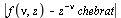 is less than
  .
.
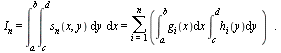
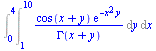
Approximation of Bivariate Functions via Tensor Product Series
Given a bivariate function  and a region of interest
 ![R = Typesetting:-delayCrossProduct([a, b], [c, d])](images/TPapprox_420.gif) , we wish to generate a numerical evaluation routine
, we wish to generate a numerical evaluation routine  such that

where  is the unit roundoff error for a specified hardware floating point precision. Moreover, the routine
  must be "purely numerical" in the sense that it can be translated into a language such as C and can be compiled for inclusion in a numerical library.
The above specification implies the need to generate numerical approximations for  . By using tensor product series approximations, the bivarate approximation problem is reduced to a sequence of univariate approximation problems and then some well-known methods for univariate approximation are applied.
As will be seen, our algorithm automatically subdivides the region  into subregions based on specified limits for the number of terms allowed in a tensor product series and for the degrees of the univariate approximations. Let us first treat a case where no subdivisions of
  are required.
Example 7.1: Tensor Product Series Approximation in a Region
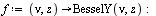
Consider the function ](images/TPapprox_428.gif) , the Bessel function of the second kind, and suppose that we approximate this function in the region
, the Bessel function of the second kind, and suppose that we approximate this function in the region ![R = Typesetting:-delayCrossProduct([1, 2], [`/`(1, 4), `/`(1, 2)])](images/TPapprox_429.gif) , in other words
, in other words  . This is a small region and no subdivisions of
  are required.
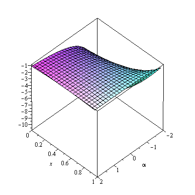
The algorithm computes a tensor product series approximation based on the following distribution of splitting points.
The matrix-vector representation of the tensor product series is as follows (carrying only 6 digits for this illustration).

![`assign`(W, Vector([seq(f(a[i], z), i = 1 .. nTerms)]))](images/TPapprox_435.gif)
](images/TPapprox_436.gif) |
(7.1.1) |
![`assign`(V, Vector([seq(f(nu, b[i]), i = 1 .. nTerms)]))](images/TPapprox_437.gif)
](images/TPapprox_438.gif) |
(7.1.2) |
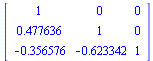
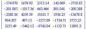
![`assign`(L, Matrix(nTerms, nTerms, [[1., 0., 0., 0., 0., 0., 0., 0., 0.], [-.228416, 1., 0., 0., 0., 0., 0., 0., 0.], [-.448593, -.685157, 1., 0., 0., 0., 0., 0., 0.], [-.206213, -1.38167, .646485, 1....](images/TPapprox_439.gif)
![`assign`(L, Matrix(nTerms, nTerms, [[1., 0., 0., 0., 0., 0., 0., 0., 0.], [-.228416, 1., 0., 0., 0., 0., 0., 0., 0.], [-.448593, -.685157, 1., 0., 0., 0., 0., 0., 0.], [-.206213, -1.38167, .646485, 1....](images/TPapprox_440.gif)
![`assign`(L, Matrix(nTerms, nTerms, [[1., 0., 0., 0., 0., 0., 0., 0., 0.], [-.228416, 1., 0., 0., 0., 0., 0., 0., 0.], [-.448593, -.685157, 1., 0., 0., 0., 0., 0., 0.], [-.206213, -1.38167, .646485, 1....](images/TPapprox_441.gif)
![`assign`(L, Matrix(nTerms, nTerms, [[1., 0., 0., 0., 0., 0., 0., 0., 0.], [-.228416, 1., 0., 0., 0., 0., 0., 0., 0.], [-.448593, -.685157, 1., 0., 0., 0., 0., 0., 0.], [-.206213, -1.38167, .646485, 1....](images/TPapprox_442.gif)
![`assign`(L, Matrix(nTerms, nTerms, [[1., 0., 0., 0., 0., 0., 0., 0., 0.], [-.228416, 1., 0., 0., 0., 0., 0., 0., 0.], [-.448593, -.685157, 1., 0., 0., 0., 0., 0., 0.], [-.206213, -1.38167, .646485, 1....](images/TPapprox_443.gif)
![`assign`(L, Matrix(nTerms, nTerms, [[1., 0., 0., 0., 0., 0., 0., 0., 0.], [-.228416, 1., 0., 0., 0., 0., 0., 0., 0.], [-.448593, -.685157, 1., 0., 0., 0., 0., 0., 0.], [-.206213, -1.38167, .646485, 1....](images/TPapprox_444.gif)
![`assign`(L, Matrix(nTerms, nTerms, [[1., 0., 0., 0., 0., 0., 0., 0., 0.], [-.228416, 1., 0., 0., 0., 0., 0., 0., 0.], [-.448593, -.685157, 1., 0., 0., 0., 0., 0., 0.], [-.206213, -1.38167, .646485, 1....](images/TPapprox_445.gif)
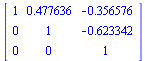
![`assign`(U, Matrix(nTerms, nTerms, [[1., -.262852, -.420037, .112824, -.267711, 0.668780e-1, -.218056, 0.699279e-1, -0.280877e-1], [0., 1., -.707500, -.549318, -0.144255e-1, -.325081, -.134516, -0.860...](images/TPapprox_455.gif)
![`assign`(U, Matrix(nTerms, nTerms, [[1., -.262852, -.420037, .112824, -.267711, 0.668780e-1, -.218056, 0.699279e-1, -0.280877e-1], [0., 1., -.707500, -.549318, -0.144255e-1, -.325081, -.134516, -0.860...](images/TPapprox_456.gif)
![`assign`(U, Matrix(nTerms, nTerms, [[1., -.262852, -.420037, .112824, -.267711, 0.668780e-1, -.218056, 0.699279e-1, -0.280877e-1], [0., 1., -.707500, -.549318, -0.144255e-1, -.325081, -.134516, -0.860...](images/TPapprox_457.gif)
![`assign`(U, Matrix(nTerms, nTerms, [[1., -.262852, -.420037, .112824, -.267711, 0.668780e-1, -.218056, 0.699279e-1, -0.280877e-1], [0., 1., -.707500, -.549318, -0.144255e-1, -.325081, -.134516, -0.860...](images/TPapprox_458.gif)
![`assign`(U, Matrix(nTerms, nTerms, [[1., -.262852, -.420037, .112824, -.267711, 0.668780e-1, -.218056, 0.699279e-1, -0.280877e-1], [0., 1., -.707500, -.549318, -0.144255e-1, -.325081, -.134516, -0.860...](images/TPapprox_459.gif)
![`assign`(U, Matrix(nTerms, nTerms, [[1., -.262852, -.420037, .112824, -.267711, 0.668780e-1, -.218056, 0.699279e-1, -0.280877e-1], [0., 1., -.707500, -.549318, -0.144255e-1, -.325081, -.134516, -0.860...](images/TPapprox_460.gif)
![`assign`(U, Matrix(nTerms, nTerms, [[1., -.262852, -.420037, .112824, -.267711, 0.668780e-1, -.218056, 0.699279e-1, -0.280877e-1], [0., 1., -.707500, -.549318, -0.144255e-1, -.325081, -.134516, -0.860...](images/TPapprox_461.gif)


If one wanted the explict expression for the tensor product series ](images/TPapprox_483.gif) it is given by
it is given by
![`assign`(s[9], Typesetting:-delayDotProduct(Typesetting:-delayDotProduct(Typesetting:-delayDotProduct(Typesetting:-delayDotProduct(`^`(V, %T), U), Diag), L), W)); -1](images/TPapprox_484.gif)
However the expression is quite large and, more significantly, with the explicit expression it is impossible to evaluate to full accuracy in hardware floating point precision. The problem can be seen by the large diagonal elements appearing above, which produce a sum of terms with large values adding up to a relatively small final answer (a classical case of unstable numerical computation!).
Fortunately, by maintaining the matrix-vector formulation we obtain a stable evaluation algorithm as will be seen.
It can be verified that (when the digits are carried to hardware floating point precision):

Example 7.2: Approximating the Univariate Functions
Continuing with the approximation problem of Example 7.1, we must now compute approximations for each of the univariate functions appearing in the vectors  and
and  .
.

](images/TPapprox_489.gif) |
(7.2.1) |

](images/TPapprox_491.gif) |
(7.2.2) |
The approach taken for each univariate function is to compute a Chebyshev series on the specified interval, truncated to accuracy  . This determines the approximation degree required for the particular function and if this degree is too large (greater than degree 25) for any of the univariate functions then the corresponding interval is subdivided and the process is repeated.
Since the degrees are not too large in this case, no subdivisions are required. Noting that rational approximations are more efficient than polynomial approximations for some functions, the algorithm will compute Chebyshev-Pade approximations if they lead to approximations of smaller total degree.
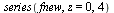
For example, consider the entry ![W[4]](images/TPapprox_493.gif) and compute a Chebyshev series to the specified accuracy. Recall from Example 6.3 that for this function it is helpful to factor out a power of
and compute a Chebyshev series to the specified accuracy. Recall from Example 6.3 that for this function it is helpful to factor out a power of  due to the singularity at
  and our algorithm will do so.
![`assign`(f, W[4])](images/TPapprox_496.gif)
 |
(7.2.3) |


 |
(7.2.4) |

 |
(7.2.5) |

 |
(7.2.6) |

 |
(7.2.7) |


 |
(7.2.9) |
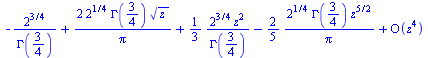
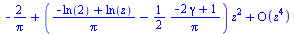
This polynomial approximation is of degree  . By trying successive Chebyshev-Pade approximants of degrees
 ![[6, 6], [5, 5], () .. ()](images/TPapprox_518.gif) decreasing until the maximum error is too large, the algorithm finds that the
decreasing until the maximum error is too large, the algorithm finds that the ![[5, 5]](images/TPapprox_519.gif) approximant (for total degree 10) achieves the desired accuracy.
approximant (for total degree 10) achieves the desired accuracy.
![`assign`(chebpad, numapprox:-chebpade(fnew, z = `/`(1, 4) .. `/`(1, 2), [5, 5]))](images/TPapprox_520.gif)
Rational approximation is advantageous over polynomial approximation for this function because, as discussed in Example 6.3, even though we have factored out a power of  to improve the leading term of the series expansion about
  , it remains the case that
  has a logarithmic singularity at
  . The left endpoint of the interval of approximation is
  which means that the singularity is "nearby".

 |
(7.2.11) |
Noting that the approximation  has been computed for the function
  , the final approximation for the original function
  is
is

In general, Chebyshev-Pade approximants will be used in this manner for the functions of  appearing in the vector
  . In contrast, for the functions of
  in the vector
  the algorithm finds that rational approximation offers no advantage and the truncated Chebyshev series is used.
For example, consider 
![V[4]](images/TPapprox_543.gif)
 |
(7.2.12) |
![`assign`(cheb, numapprox:-chebyshev(V[4], nu = 1 .. 2, hftol))](images/TPapprox_545.gif)

 |
(7.2.14) |
One finds that rational approximations offer no advantage for the univariate functions of  meaning that these functions are "polynomial-like".
Remark on Data Structures
For each univariate function appearing in  and in
  , we must store information about the corresponding polynomial or rational approximation. The most general form of approximation to be stored is the form appearing for the function
  considered above, which is of the form:

where  in that particular example and where
![chebratForm = `/`(`*`(Sum(`*`(c[k], `*`(T[k](`+`(`*`(alpha, `*`(z)), beta)))), k = 0 .. m)), `*`(Sum(`*`(d[k], `*`(T[k](`+`(`*`(alpha, `*`(z)), beta)))), k = 0 .. n)))](images/TPapprox_562.gif)
![chebratForm = `/`(`*`(Sum(`*`(c[k], `*`(T[k](`+`(`*`(alpha, `*`(z)), beta)))), k = 0 .. m)), `*`(Sum(`*`(d[k], `*`(T[k](`+`(`*`(alpha, `*`(z)), beta)))), k = 0 .. n)))](images/TPapprox_563.gif) |
(7.3.1) |
Therefore for each entry in  and in
  , we store a vector containing the following purely numerical information:
![[tau, alpha, beta, c[0], c[1], () .. (), c[m], d[0], d[1], () .. (), d[n]]](images/TPapprox_566.gif)
Evaluation of the approximation at a point ![z = z[j]](images/TPapprox_567.gif) requires evaluation of the numerator and denominator polynomials in Chebyshev form. Since there are several such polynomials in Chebyshev form (the numerator and denominator in the approximations for each entry in
requires evaluation of the numerator and denominator polynomials in Chebyshev form. Since there are several such polynomials in Chebyshev form (the numerator and denominator in the approximations for each entry in  , for example), it can be advantageous to use a vectorized form of the evaluation algorithm.
Similarly, there would be approximations of the same form for the univariate functions of ν appearing in the vector  . As noted above, in some cases the approximation will be a polynomial rather than a rational function, in which case the denominator is simply 1.
Example 7.4: Stable Evaluation of the Matrix-Vector Form
Suppose that we have stored polynomial or rational approximations for each univariate function appearing in the vectors  and
and  of the preceding Example. Given our overall approximation of the function
 ](images/TPapprox_572.gif) in the region
in the region ![R = Typesetting:-delayCrossProduct([1, 2], [`/`(1, 4), `/`(1, 2)])](images/TPapprox_573.gif) , suppose that we wish to evaluate at the point
, suppose that we wish to evaluate at the point  .
.
Since we have stored accurate approximations for the univariate functions, we will evaluate the vectors  and
and  to the following values (for simplicity here, we just enter the correct numerical values).
We will use  here for illustration, but we would normally work with hardware floating point precision. Also, for this precision the number of terms required would be
  .
.


![`assign`(V, V[1 .. nTerms]); -1; `assign`(W, W[1 .. nTerms]); -1](images/TPapprox_582.gif)
![`assign`(L, L[1 .. nTerms, 1 .. nTerms]); -1; `assign`(U, U[1 .. nTerms, 1 .. nTerms]); -1](images/TPapprox_583.gif)
![`assign`(Diag, Diag[1 .. nTerms, 1 .. nTerms]); -1](images/TPapprox_584.gif)

](images/TPapprox_587.gif) |
(7.4.1) |

](images/TPapprox_589.gif) |
(7.4.2) |
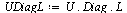
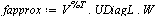
Then the tensor product series approximation in the region  has the following matrix-vector representation which can be evaluated to yield the desired numerical value.

 |
(7.4.3) |

 |
(7.4.4) |
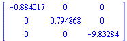
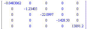
Note that  has entries which grow large and this can cause unstable numerical evaluation unless we choose the correct order of evaluation. The bracketing above specifies the correct order of evaluation.

 |
(7.4.5) |
The following is an example of unstable evaluation.
Suppose that we first compute the product of the three matrices.
 |
(7.4.6) |
 |
(7.4.7) |

 |
(7.4.8) |
This result has no correct digits!
Fortunately, using the right-to-left evaluation of the matrix-vector form can be shown to be numerically stable.
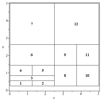
Example 7.5: Approximation in a Large Region
Consider once again the Bessel function of the second kind, ](images/TPapprox_604.gif) , but this time in a larger region
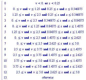
, but this time in a larger region ![R = Typesetting:-delayCrossProduct([0, 5], [`/`(1, 4), 5])](images/TPapprox_605.gif) . Our algorithm was run for this example and the region was subdivided based on the requirements:
. Our algorithm was run for this example and the region was subdivided based on the requirements:
 and
and 
where  is the number of terms in a tensor product series expansion and
  refers to the degree of the polynomials appearing in the numerator or denominator of the univariate approximations.
The algorithm produces a hash function such that, given an evaluation point ![nu[i], z[j]](images/TPapprox_610.gif) the result of
the result of ![hash(nu[i], z[j])](images/TPapprox_611.gif) is an integer index
is an integer index  into the array of numerical values defining the approximation on the
  subregion. Specifically, the hash function for this example is the following Maple
  expression indicating that the region
  was subdivided into 12 subregions.


 |
(7.5.1) |
For example, for evaluation at the point  we get

 |
(7.5.2) |
indicating that we must evaluate the approximation stored for the subregion indexed by 2.
The 12 subregions for the above example are pictured in the plot below.
As can be seen, the individual subregions have index numbers ranging from 1 to 12.
References
[Carvajal04] O.A. Carvajal, A New Hybrid Symbolic-Numeric Method for Multiple Integration Based on Tensor-Product Series. Master's thesis, School of Computer Science, University of Waterloo, 2004.
[CarvajalChapmanGeddes05] O.A. Carvajal, F.W. Chapman and K.O. Geddes, Hybrid symbolic-numeric integration in multiple dimensions via tensor-product series. Proc. ISSAC'05, Manuel Kauers (ed.), ACM Press, New York, 2005, pp. 84-91.
[Chapman03] F.W. Chapman, Generalized Orthogonal Series for Natural Tensor Product Interpolation. Ph.D thesis, Department of Applied Mathematics, University of Waterloo, 2003.
[Davis63] P.J. Davis, Interpolation and Approximation. Blaisdell, 1963.
[Thomas76] D.H. Thomas, A natural tensor product interpolation formula and the pseudoinverse of a matrix. Linear Algebra and Its Applications, 1976.
[Wang08] Xiang Wang, Automated Generation of Numerical Evaluation Routines for Bivariate Functions via Tensor Product Series. Master's thesis, School of Computer Science, University of Waterloo, 2008.
](images/TPapprox_210.gif)
](images/TPapprox_212.gif)