A Package for Numerical Approximation 

K.O. Geddes
Symbolic Computation Group
University of Waterloo 

Preface 

A package named ``numapprox'' was introduced in Maple V Release 2.  This package contains various procedures for developing numerical approximations of functions.  Examples of its use are presented here using the Maple worksheet facility. 

>

restart;

 

>	with(numapprox);

 

(1)

 

>

 

We will use several of these procedures to develop numerical approximations for a particular mathematical function.  The mathematical function which we wish to approximate is the function discussed in section 6.9 of the book First Leaves: A Tutorial Introduction to Maple V.  The function is as follows. 

>	f := x -> int(1/GAMMA(t), t=0..x ) / x^2;

 

(2)

 

>

 

Numerical evaluation of f(x) is quite expensive because it requires a numerical integration computation for each particular value x.  Hence many of the computations in this session require a nontrivial amount of execution time.  The purpose of the exercise is to develop efficient evaluation procedures for f(x) by computing polynomial and rational function approximations for f(x).  Our ultimate goal is to develop an evaluation procedure which yields six digits of accuracy and which requires the fewest possible number of arithmetic operations for each evaluation. 

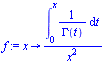
A plot of f(x) appears as follows. 

>	plot(f, 0..4);

 

>

 

Approximations derived from Taylor series 

Efficient evaluation procedures are usually based on polynomial approximations or rational function approximations (i.e. quotients of polynomials).  The reason is that a polynomial or a rational function can be evaluated directly using only the four basic arithmetic operations:  addition, subtraction, multiplication, and division. 

As our first approximation to the function f(x), we compute the Taylor polynomial of degree 8 about the midpoint of the interval. 

>	s := map(evalf, taylor(f(x), x=2, 9));

 

(3)

 

>

 

For convenience, we convert the approximation to functional form to correspond with the form specified for the original function f.  Then we plot the error curve for this Taylor polynomial approximation. 

>	TaylorApprox := convert(s, polynom):

 

>	TaylorApprox := unapply(TaylorApprox, x);

 

(4)

 

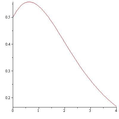
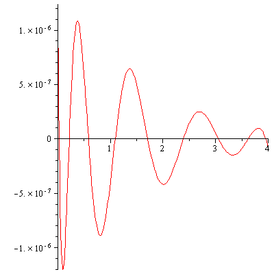
The error curve for this Taylor polynomial approximation takes the following form. 

>	plot(f - TaylorApprox, 0..4);

 

>

 

It is a typical property of Taylor approximations that the error is small near the point of the Taylor series expansion and the error gets larger as the distance from the point of expansion increases.  In this particular case, the largest error occurs at the left endpoint. 

To compute the value of the error at x=0, note that direct evaluation of f(0) will lead to a division by zero (see the definition of f) so we must use a limit value. 

>	maxTaylorError := abs( limit(f(x), x=0) - TaylorApprox(0) );

 

(5)

 

>

 

Pade approximation 

Next we compute the Pade rational approximation of degree (4,4) for f(x).  The approximations being computed for the remainder of this session will approximate the function more accurately and roundoff errors in the calculations will become significant.  Therefore, we will now do the calculations carrying two extra digits of precision. 

>	Digits := 12:

 

>	s := map(evalf, taylor(f(x), x=2, 9)):

 

>	PadeApprox := pade(s, x=2, [4,4]);

 

(6)

 

>	PadeApprox := unapply(PadeApprox, x):

 

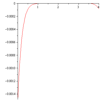
The error curve for the (4,4) Pade approximation takes the following form. 

>	plot(f - PadeApprox, 0..4);

 

>

 

As with Taylor polynomial approximations, it is a typical property of Pade approximations that the error is small near the point of expansion and the error gets larger as the distance from the point of expansion increases.  Again we see from the plot that for this particular function, the largest error occurs at the left endpoint. 

However, we find that the maximum error in the Pade approximation is an order of magnitude smaller than the maximum error in the corresponding Taylor polynomial approximation. 

>	maxPadeError := abs( limit(f(x), x=0) - PadeApprox(0) );

 

(7)

 

>

 

Approximations derived from Chebyshev series 

In general, better approximations on an interval can be obtained using Chebyshev series expansions rather than Taylor series expansions.  The Chebyshev series expansion of f(x) on [0,4] is as follows, where we specify that we want accuracy 1E-8 which means that all terms with coefficients smaller than this magnitude will be dropped.  We discover that this yields a degree 13 approximation. 

>	evalf( limit(f(x), x=0) );

 

(8)

 

>	fproc := proc(x) if x=0 then 0.5 else evalf(f(x)) fi end:

 

>	ChebApprox := chebyshev(fproc, x=0..4, 1E-8);

 

(9)

 

>

 

If the error in a Chebyshev series approximation is plotted, it typically shows an oscillating error curve as can be verified for this example (see the First Leaves reference mentioned above).  If the Chebyshev series was truncated at degree 8, to yield a polynomial with the same degree as the Taylor polynomial approximation considered above, we would find that the maximium error in the Chebyshev series approximation of degree 8 is approximately 0.6E-5.  This is two orders of magnitude smaller than the error in the (4,4) Pade approximation computed above. 

For subsequent calculations, it is useful to note that we can use a procedure for computing numerical values of f(x) which will be much less expensive than the direct definition, which requires a numerical integration process for each specific value.  Namely, let us define a numerical evaluation procedure based on the Chebyshev series of degree 13 since the maximum error in ChebApprox is less than 1E-8, sufficient accuracy for our purposes.  We give T its polynomial definition from the orthopoly package and then we convert the polynomial to Horner (nested multiplication) form for efficient evaluation. 

>	F := hornerform( eval(subs(T=orthopoly[T], ChebApprox)) );

 

(10)

 

>	F := unapply(F, x):

 

>

 

Chebyshev-Pade approximation 

Just as we found that going from a Taylor polynomial to a Pade rational function yielded a more accurate approximation, it is equally useful to consider a Chebyshev-Pade rational approximation.  The (m,n) Chebyshev-Pade approximation for f(x) is a rational function r[m,n](x) with numerator of degree m and denominator of degree n such that the Chebyshev series expansion of r[m,n](x) agrees with the Chebyshev series expansion of f(x) through the term of degree m+n. 

We compute the Chebyshev-Pade approximation of degree (4,4) to correspond with the Pade approximation computed earlier. 

>	ChebPadeApprox := chebpade(F,  0..4, [4,4]);

 

(11)

 

>	with(orthopoly, T):

 

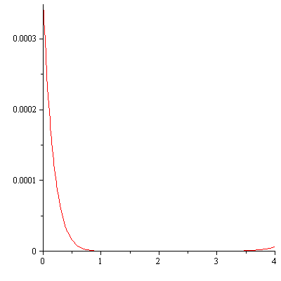
>	plot(F - ChebPadeApprox, 0..4);

 

>

 

The maximum error occurs, once again, at the left endpoint.  The magnitude of the maximum error is somewhat smaller than the error in the corresponding Chebyshev series approximation.  The main advantage of the rational function form is the efficiency of evaluation which can be achieved by converting to continued fraction form (see below). 

>	maxChebPadeError :=  abs( F(0) - ChebPadeApprox(0) );

 

(12)

 

>

 

Minimax approximation 

It is a classical result of Approximation Theory that the best minimax rational function approximation of degree (m,n) is achieved when the error curve has m+n+2 oscillations which are equal in magnitude.  The error curve of the Chebyshev-Pade approximation has the correct number of oscillations but its error curve must be ``levelled'' in order to achieve the best minimax approximation.  This task is achieved by the minimax procedure. 

>	MinimaxApprox := minimax(F, 0..4, [4,4], 1, 'maxerror');

 

(13)

 

>

 

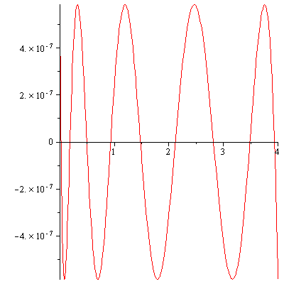
The maximum error in MinimaxApprox is given by the value of the variable maxerror.  It can be seen that we have achieved our goal of obtaining an approximation with error less than 1E-6.  A plot of the error curve displays the predicted property of equal oscillations. 

>	maxMinimaxError := maxerror;

 

(14)

 

>	plot(F - MinimaxApprox, 0..4);

 

>

 

Efficient evaluation of rational functions 

The numerator and denominator polynomials in MinimaxApprox have already been expressed in Horner form (i.e. nested multiplication form).  The cost of evaluating a polynomial of degree n in Horner form is n multiplications and n additions and this is the most efficient evaluation scheme for a general polynomial. 

However, for a rational function of degree (m,n) we can do better than simply expressing each of numerator and denominator in Horner form.  Noting that we could normalize the rational function such that the denominator polynomial is monic (i.e. leading coefficient 1), to save one multiplication operation, we can see that the cost of evaluating a rational function of degree (m,n) in Horner form is m+n additions, m+n-1 multiplications, and 1 division.  In other words, the total operation count is 

    m+n multiplication/division operations, 

    m+n addition/subtraction operations. 

The cost of evaluating a rational function can be reduced significantly by converting it to continued fraction form.  Specifically, a rational function of degree (m,n) can be evaluated using at most 

    max(m,n) multiplication/division operations, 

    m+n addition/subtraction operations. 

For example, if m=n then this new scheme requires only half the number of multiplication/division operations compared with the preceding method. 

For the rational function MinimaxApprox, the cost of evaluation in the form expressed above is 9 multiplication/division operations and 8 addition/subtraction operations.  (The 9 could be reduced to 8 simply by normalizing to make the denominator monic.)  We now compute the continued fraction form for this same rational function and it can be seen from the output that the cost of evaluation in this form is only 4 division operations and 8 addition/subtraction operations. 

>	MinimaxApprox := confracform(MinimaxApprox):

 

>	lprint(MinimaxApprox(x));

 

-0.468861423888e-1+1.07859145304/(x+4.41993680008+16.1901824390/(x+4.29117629353+70.1940954307/(x-10.2912368965+4.77540461444/(x+1.23883867138))))

 

>

 

Timing comparisons 

We now time the actual cost to evaluate the function f(x) at 1000 points using the original integral definition and compare it with the cost to evaluate MinimaxApprox in continued fraction form.  Since our approximation will yield only 6 digits of accuracy, we only ask for 6 digits of accuracy from the integral definition as well. 

>	Digits := 6:  st := time():

 

>	seq( evalf(f(i/250.0)), i = 1..1000 ):

 

>	oldtime := time() - st;

 

(15)

 

The continued fraction form of a rational function sometimes requires that a few extra guard digits be carried during evaluation.  In this case, it is sufficient to carry two extra digits.  We find that the evaluation procedure based on MinimaxApprox is more than 150 times faster than evaluating the original integral definition. 

>	Digits := 8:  st := time():

 

>	seq( MinimaxApprox(i/250.0), i = 1..1000 ):

 

>	newtime := time() - st;

 

(16)

 

>	SpeedUp := oldtime/newtime;

 

(17)

 

>

 

Conversion to FORTRAN or C code 

One of the common reasons for developing an efficient numerical evaluation procedure for a mathematical function is for the purpose of including it in a subroutine library in some other language such as FORTRAN or C.  Conversion routines are available in Maple to convert to either of these languages.  As an example, we convert the formula for MinimaxApprox into FORTRAN syntax. 

>	codegen:-fortran(MinimaxApprox(x));

 

t0 = -0.468861423888D-1+0.107859145304D1/(x+0.441993680008D1+0.161

 

#90182439D2/(x+0.429117629353D1+0.701940954307D2/(x-0.102912368965D     #2+0.477540461444D1/(x+0.123883867138D1))))

 

>

 

Concluding remarks 

We have shown how the facilities in Maple can be used very effectively to develop procedures for the efficient numerical evaluation of mathematical functions.  Specifically, the ability to generate series expansions, to compute rational function approximations, and to convert to various special forms, combined with the powerful interactive tool of viewing plots of the approximations and their error curves, provides an ideal environment for such tasks. 

This complete article, including Maple input, output, text, and graphics, was created and formatted as an interactive Maple worksheet. 

>