Banquet06.html

Banquet06.mw

25 Years of Maple:
Some Historical Comments

Keith Geddes
Maple Conference 2006

In the Beginning

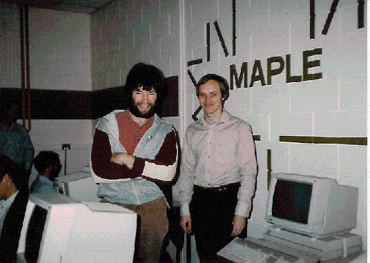
In the beginning (1980) there were two of us: Gaston Gonnet and Keith Geddes

Pre-Maple

1970s: I specialized in Numerical Analysis (Approximation Theory)

Began to use early systems for Computer Algebra

in those days we called it "symbolic computation"

or "algebraic manipulation"

Witness: ACM SIGSAM (for "symbolic and algebraic manipulation")

The computers were "large" (but lacking in speed and memory space!!)

The "red room" in the Math and Computer building at UW

Early Computer Algebra Systems

I used various CA systems in the 1970s

for teaching and research work

Formac (a preprocessor to PL/1)

batch processing

ALTRAN (a preprocessor to Fortran)

very Fortran-like programming

batch processing

restricted to polynomial and rational function manipulation

Communicate to the mainframe from a terminal

I recall the so-called "silent 700"
(not very silent, but compared to an IBM 2741 type-ball terminal!)

I had a Teleterm terminal
(cost $5200 in 1974)

connect to campus mainframe at 300 baud

The issue of memory size

we used a Honeywell time-sharing mainframe

50K words (i.e., 200K bytes) of memory usage was "very large"

often wait overnight for processing to finish

would lead to high charges to my research grant

could not use more than a half-megabyte of memory

How large do integers need to be?

For example, compute the GCD of two polynomials

In ALTRAN, max length for integers was 100 digits
(this is the maximum that could be requested!)

100 digits sounds "large enough" for many purposes

The Problem: Intermediate steps of an algorithm may generate very large integers
(using the only GCD algorithms known at the time)

The GCD algorithm used was a variation of the ancient Euclid algorithm (based on PRS, meaning Polynomial Remainder Sequences)

The computation is ridiculously trivial in modern times!
(with modern algorithms as well as fast computers)

(1)

(2)

(3)

Note: The maximum length of integers above is 10 digits.

The old algorithm `gcd/reduced` (which uses a PRS algorithm) yields the same result. It even seems fast enough on modern computers.However, notice the large integers that can be generated by intermediate calculations!

We very soon ran into GCD computations that could not be completed on a system that limits the size of integers to only 100 digits.

(4)

{--> enter gcd/reduced, args = 2500000*x^4-487995500*x^3-2442003501*x^2+308523500*x+4504301, 125000*x^3+1110250*x^2+2426470*x+2501
{--> enter gcd/reduced/prs, args = 2500000*x^4-487995500*x^3-2442003501*x^2+308523500*x+4504301, 125000*x^3+1110250*x^2+2426470*x+2501

{--> enter gcd/reduced/prs, args = 2500000, 487995500

<-- exit gcd/reduced/prs (now in gcd/reduced/content) = 500}
{--> enter gcd/reduced/prs, args = 500, 2442003501

<-- exit gcd/reduced/prs (now in gcd/reduced/content) = 1}

{--> enter gcd/reduced/prs, args = 125000, 1110250

<-- exit gcd/reduced/prs (now in gcd/reduced/content) = 250}
{--> enter gcd/reduced/prs, args = 250, 2426470

<-- exit gcd/reduced/prs (now in gcd/reduced/content) = 10}
{--> enter gcd/reduced/prs, args = 10, 2501

<-- exit gcd/reduced/prs (now in gcd/reduced/content) = 1}

{--> enter gcd/reduced/prs, args = 1, 1

<-- exit gcd/reduced/prs (now in gcd/reduced/prs) = 1}

{--> enter gcd/reduced/prs, args = 12931048027941398437500000000000, 64681102235762874984375000000000

<-- exit gcd/reduced/prs (now in gcd/reduced/content) = 25862096055882796875000000000}

<-- exit gcd/reduced/prs (now in gcd/reduced) = 2501+500*x}

<-- exit gcd/reduced (now at top level) = 2501+500*x}

(5)

The point of the above trace of a computation: Large intermediate integers arise, much larger than the size of integers in the input and the output

By the late 1970s, I made some use of MACSYMA

Developed at MIT

How did I use it?
By dialing long-distance to a DEC 10 computer at MIT in Boston

My question to my Computer Science colleagues:

How can we get a computer that would run MACSYMA at U of Waterloo?

My colleagues answer: That is the wrong question!

1980: The Age of Maple arrives!

I was on sabbatical at Berkeley during the first half of 1980, hosted by Richard Fateman

started writing a textbook on algebraic algorithms

which eventually got completed (with co-authors) in 1992 :

But back to 1980!

I called a meeting of my CS colleagues at UW in November 1980

My question: Can we apply for research grant to buy a computer large enough to run MACSYMA?

The answer (typical of UW): You should build your own system, and (avoiding LISP as an implementation language) try to do much more with fewer computing resources.

In short, using a BCPL-language (eventually, this meant the C language) we did develop the Maple system which could do more with less!

It was at this November 1980 meeting where I learned that fellow faculty member, Gaston Gonnet, was also interested in algebraic computation.

Gaston had already developed a mini-CA system (WAMA -- Waterloo Algebraic Manipulation) during 1979-80, for doing asymptotic analysis calculations related to the analysis of algorithms.

By the first week of December 1980, Gaston had put together the first running system to which we gave the name "Maple".

Where does the name "Maple" come from?
It is just a Canadian name -- after first thinking of acronyms for "Mathematical Programming Language", for example.

Now I could proceed with my interest in "Algorithms for Computer Algebra" by implementing the algorithms in Maple.

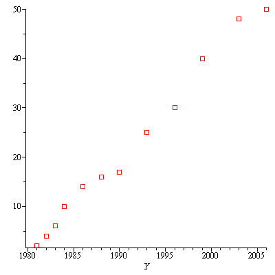
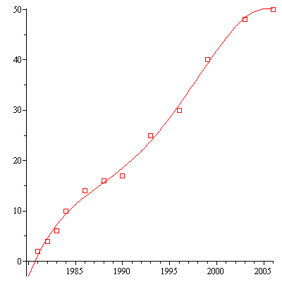
How many Person-Years of R&D for Maple?

Start date is 1 Dec 1980.

Of course, we need a Maple calculation to figure out the number of person-years of R&D effort.

Note: The numbers for PersonsPerYear below are fictitious -- but maybe something like this!

Plot_2d

(6)

(7)

(8)

(9)

Plot_2d

(10)

Voila!

1981-1985

Michael Monagan and Greg Fee

Michael Monagan arrived at UW (from New Zealand) as a graduate student in 1982.

By the end of the 1980s when we needed to calculate the contributions to Maple code by various authors, Michael was one of the "top three" contributors (Gaston, Keith and Michael) -- in some order (I believe that Michael was ahead of one or both of us).

Michael's contributions have been at the level of the Maple kernel code as well as external library code.

... and his contributions keep coming!

Greg Fee and Benton Leong were hired to work on the Maple project about 1981 and remained with the project for many years.

Benton Leong and Howard Johnson

A good view of the "ASCII Maple logo"

Credit for inventing the "ASCII Maple logo" goes to Stephen Watt, who completed his PhD degree under my supervision in the early 1980s.

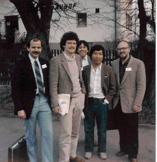
Stan Devitt, Stephen Watt, Bruce Char, Benton Leong, Keith Geddes

(in Linz, Austria for the 1985 Eurocal conference)

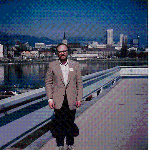
A geeky picture of me in Linz, Austria (1985)

1986-2006: More Pictures

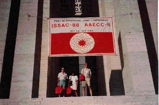
ISSAC '88 in Rome -- the first to be named "ISSAC"

Rome 1988

Bruce Char and Mark Mutrie, Maple Retreat 1989

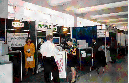
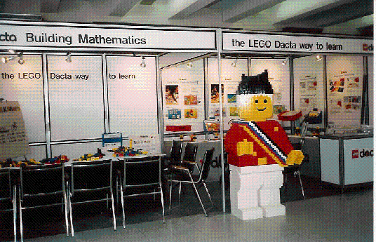
Maple booth, NCTM 1992, Quebec City

A view of the competition, NCTM 1992, Quebec City

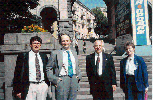
Stephen Watt and I with hosts, Kiev 1993

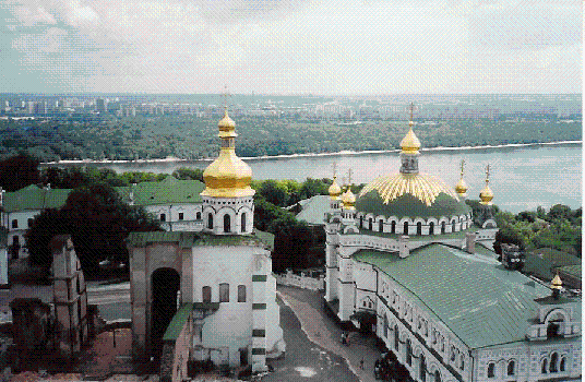
Kiev 1993

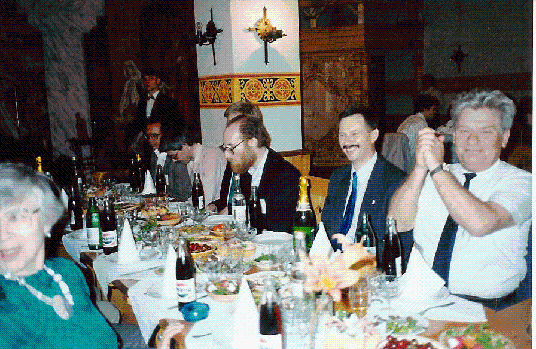
The vodka banquet, Kiev 1993

W. Kahan, K. Geddes, D. Jeffrey, G. Labahn, Ha Le, Maple Retreat 1994

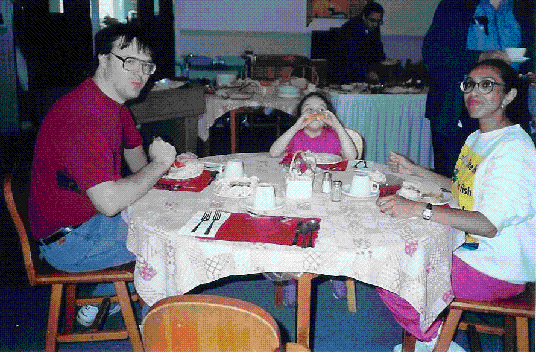
Rob Corless family, Maple Retreat 1994

G. Gonnet, B. Salvy, M. Bronstein, Maple Retreat 1994

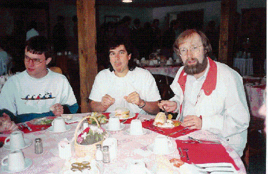
Erich Kaltofen with Allan Bonadio and ??, Maple Retreat 1994

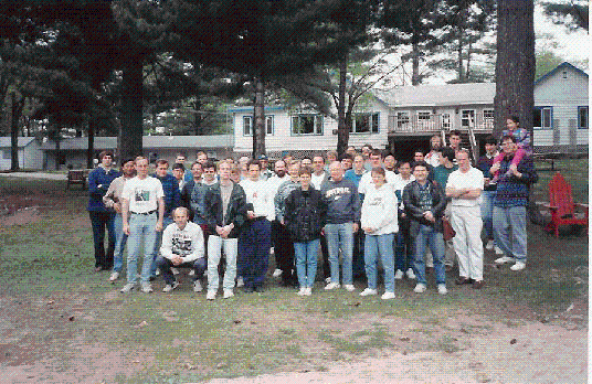
Group picture, Maple Retreat 1994

Hard at work at the Maple Retreat, Sparrow Lake, Ontario, 1997

A view outside the ISSAC '97 conference, Maui, Hawaii

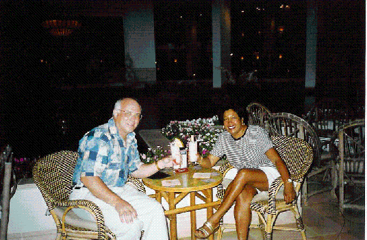
Keith and Debbie, ISSAC '97, Maui, Hawaii

{--> enter gcd/reduced, args = 2500000x^4-487995500x^3-2442003501x^2+308523500x+4504301, 125000x^3+1110250x^2+2426470x+2501 {--> enter gcd/reduced/prs, args = 2500000x^4-487995500x^3-2442003501x^2+308523500x+4504301, 125000x^3+1110250x^2+2426470x+2501





{--> enter gcd/reduced/prs, args = 2500000, 487995500


<-- exit gcd/reduced/prs (now in gcd/reduced/content) = 500} {--> enter gcd/reduced/prs, args = 500, 2442003501


<-- exit gcd/reduced/prs (now in gcd/reduced/content) = 1}

{--> enter gcd/reduced/prs, args = 125000, 1110250


<-- exit gcd/reduced/prs (now in gcd/reduced/content) = 250} {--> enter gcd/reduced/prs, args = 250, 2426470


<-- exit gcd/reduced/prs (now in gcd/reduced/content) = 10} {--> enter gcd/reduced/prs, args = 10, 2501


<-- exit gcd/reduced/prs (now in gcd/reduced/content) = 1}

{--> enter gcd/reduced/prs, args = 1, 1


<-- exit gcd/reduced/prs (now in gcd/reduced/prs) = 1}










{--> enter gcd/reduced/prs, args = 12931048027941398437500000000000, 64681102235762874984375000000000


<-- exit gcd/reduced/prs (now in gcd/reduced/content) = 25862096055882796875000000000}

<-- exit gcd/reduced/prs (now in gcd/reduced) = 2501+500*x}

<-- exit gcd/reduced (now at top level) = 2501+500*x}
	(5)