AfterDinner07.mw

Symbolic-Numeric Reflections:
One Person's 35-year Perspective
 

Keith Geddes

SNC '07
The University of Western Ontario
27 July 2007
 

Abstract 

This will be an informal after-dinner talk recalling some events of past years related to scientific computation and computer algebra. 

What this is not: This is not a comprehensive overview of historical developments in numerical analysis and computer algebra, nor of the development of "symbolic-numeric computation". 

It is more casual and light-hearted (as expected for an after-dinner talk), but with some mention of significant historical developments. 


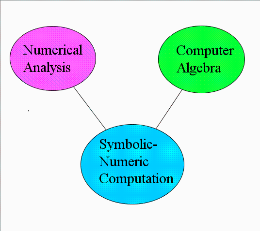
The SNC Landscape 


Drawing-Canvas 


Approximate Timelines 


  • Numerical Analysis:  Approx. 1950 to the present
 

  • Computer Algebra:  Approx. 1960 to the present
 

  • Symbolic-Numeric Computation:  Approx. 1990 to the present


My Personal Timelines 


  • 1970s:  Numerical Analysis

    - PhD Thesis,
    Algorithms for Analytic Approximation, 1973

    - My 1970s papers primarily in Numerical Approximation
     with particular interest in
     - Chebyshev series
     - Chebyshev-Pade approximation
     - Clenshaw-Curtis quadrature
 

  • 1980s:  Computer Algebra

    - The Maple project, started about November 1980

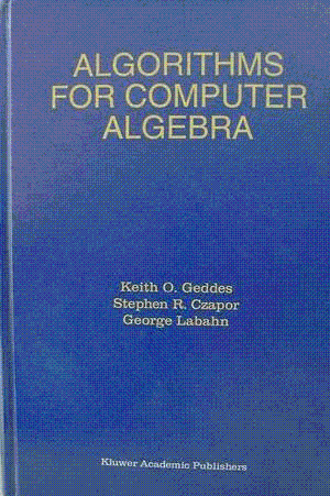
    - Textbook,
    Algorithms for Computer Algebra (Geddes, Czapor, Labahn),
       publication date 1992
 

  • 1990s and 2000s:  More emphasis on Symbolic-Numeric Computation

    - Numerical integration using symbolic analysis,
       incorporated into Maple's numerical integration facility

    - Recent work with former PhD student Fred Chapman
       on
    bivariate approximation
       also
    numerical multidimensional integration


Early Milestones related to SNC 


J. H. Wilkinson 

  • Rounding Errors in Algebraic Processes, 1963
 

  • The Algebraic Eigenvalue Problem, 1965


Key concepts: 

  • introduced backward error analysis
 

  • also numerically stable algorithms for eigenproblems


W. Kahan 

Among many contributions, I mention 

  • Conserving Confluence Curbs Ill-Condition, 1972 Tech Rep (Berkeley)


Key concepts: 

  • root-finding becomes ill-conditioned for multiple or nearly-equal roots but
 

  • determining the location of an m-fold cluster of roots is well-conditioned


B. Buchberger 

  • An Algorithm for Finding a Basis for the Residue Class Ring of a Zero-Dimensional Polynomial Ideal (German), PhD Thesis, 1965
 

  • subsequent papers in the 1970s, 1980s, etc.


Key concept: 

  • Groebner bases


The Maple Project: Some recollections 

Pre-Maple 

  • In the 1970s I used early systems for Computer Algebra
    - for teaching and research work
 

  • In those days we called it "symbolic computation"
 

  • or "algebraic manipulation"
 

  • Witness: ACM SIGSAM (for "symbolic and algebraic manipulation")


  • The computers were "large" (but lacking in speed and memory space!!)


Image 


The "red room" in the Math and Computer building at UW 


Early Computer Algebra Systems 


  • Formac (a preprocessor to PL/1)
 

  • batch processing


  • ALTRAN (a preprocessor to Fortran)
 

  • very Fortran-like programming
 

  • batch processing
 

  • restricted to polynomial and rational function manipulation


  • Communicate to the mainframe from a terminal
 

  • I recall the so-called "silent 700"
    (not very silent, but compared to an IBM 2741 type-ball terminal!)
 

  • I had a Teleterm terminal
    (cost $5200 in 1974)
 

  • connect to campus mainframe at 300 baud


  • The issue of memory size
 

  • we used a Honeywell time-sharing mainframe
 

  • 50K words (i.e., 200K bytes) of memory usage was "very large"
 

  • often wait overnight for processing to finish
 

  • would lead to high charges to my research grant
 

  • could not use more than a half-megabyte of memory


How large do integers need to be? 


  • For example, compute the GCD of two polynomials
 

  • In ALTRAN, max length for integers was 100 digits
    (this is the maximum that could be requested!)
 

  • 100 digits sounds "large enough" for many purposes
 

  • The Problem: Intermediate steps of an algorithm may generate very large integers
    (using the only GCD algorithms known at the time)
 

  • The GCD algorithm used was a variation of the ancient Euclid algorithm (based on PRS, meaning Polynomial Remainder Sequences)
 

  • The computation is ridiculously trivial in modern times!
    (with
    modern algorithms as well as fast computers)
 

> `assign`(poly1, `+`(`*`(2500000, `*`(`^`(x, 4))), `-`(`*`(487995500, `*`(`^`(x, 3)))), `-`(`*`(2442003501, `*`(`^`(x, 2)))), `*`(308523500, `*`(x)), 4504301)); -1
 

> `assign`(poly2, `+`(`*`(125000, `*`(`^`(x, 3))), `*`(1110250, `*`(`^`(x, 2))), `*`(2426470, `*`(x)), 2501)); -1
 

> gcd(poly1, poly2)
 

`+`(2501, `*`(500, `*`(x))) (1)


Note: The maximum length of integers above is 10 digits. 


The old algorithm `gcd/reduced` (which uses a PRS algorithm) yields the same result. It even seems fast enough on modern computers.However, notice the large integers that can be generated by intermediate calculations!
 

We very soon ran into GCD computations that could not be completed on a system that limits the size of integers to only 100 digits. 


> trace(`gcd/reduced`, `gcd/reduced/prs`); -1
 

> `gcd/reduced`(poly1, poly2)


{--> enter gcd/reduced, args = 2500000*x^4-487995500*x^3-2442003501*x^2+308523500*x+4504301, 125000*x^3+1110250*x^2+2426470*x+2501


{--> enter gcd/reduced/prs, args = 2500000*x^4-487995500*x^3-2442003501*x^2+308523500*x+4504301, 125000*x^3+1110250*x^2+2426470*x+2501
{x}
x
`+`(`*`(2500000, `*`(`^`(x, 4))), `-`(`*`(487995500, `*`(`^`(x, 3)))), `-`(`*`(2442003501, `*`(`^`(x, 2)))), `*`(308523500, `*`(x)), 4504301)
`+`(`*`(125000, `*`(`^`(x, 3))), `*`(1110250, `*`(`^`(x, 2))), `*`(2426470, `*`(x)), 2501)
1
{--> enter gcd/reduced/prs, args = 2500000, 487995500
{}
500
<-- exit gcd/reduced/prs (now in gcd/reduced/content) = 500}
{--> enter gcd/reduced/prs, args = 500, 2442003501
{}
1
<-- exit gcd/reduced/prs (now in gcd/reduced/content) = 1}
`+`(`*`(2500000, `*`(`^`(x, 4))), `-`(`*`(487995500, `*`(`^`(x, 3)))), `-`(`*`(2442003501, `*`(`^`(x, 2)))), `*`(308523500, `*`(x)), 4504301)
{--> enter gcd/reduced/prs, args = 125000, 1110250
{}
250
<-- exit gcd/reduced/prs (now in gcd/reduced/content) = 250}
{--> enter gcd/reduced/prs, args = 250, 2426470
{}
10
<-- exit gcd/reduced/prs (now in gcd/reduced/content) = 10}
{--> enter gcd/reduced/prs, args = 10, 2501
{}
1
<-- exit gcd/reduced/prs (now in gcd/reduced/content) = 1}
`+`(`*`(125000, `*`(`^`(x, 3))), `*`(1110250, `*`(`^`(x, 2))), `*`(2426470, `*`(x)), 2501)
{--> enter gcd/reduced/prs, args = 1, 1
{}
1
<-- exit gcd/reduced/prs (now in gcd/reduced/prs) = 1}
1
`+`(229881134437500000, `*`(31891686562500000000, `*`(`^`(x, 2))), `*`(159568174029375000000, `*`(x)))
`+`(`*`(125000, `*`(`^`(x, 3))), `*`(1110250, `*`(`^`(x, 2))), `*`(2426470, `*`(x)), 2501)
true
15625000000
`+`(`-`(1010642222433794921630859375000000000000000), `-`(`*`(202047625436584350585937500000000000000000, `*`(x))))
`+`(229881134437500000, `*`(31891686562500000000, `*`(`^`(x, 2))), `*`(159568174029375000000, `*`(x)))
true
1017079671800743066406250000000000000000
0
{--> enter gcd/reduced/prs, args = 12931048027941398437500000000000, 64681102235762874984375000000000
{}
25862096055882796875000000000
<-- exit gcd/reduced/prs (now in gcd/reduced/content) = 25862096055882796875000000000}
`+`(2501, `*`(500, `*`(x)))
<-- exit gcd/reduced/prs (now in gcd/reduced) = 2501+500*x}
`+`(2501, `*`(500, `*`(x)))
<-- exit gcd/reduced (now at top level) = 2501+500*x}
`+`(2501, `*`(500, `*`(x))) (2)
 

>


  • The point of the above trace of a computation: Large intermediate integers arise, much larger than the size of integers in the input and the output


  • By the late 1970s, I made some use of MACSYMA
 

  • Developed at MIT
 

  • How did I use it?
    By dialing long-distance to a DEC 10 computer at MIT in Boston


  • My question to my Computer Science colleagues:
 

  • How can we get a computer that would run MACSYMA at U of Waterloo?
 

  • My colleagues answer: That is the wrong question!
 

1980: The Maple Project Begins 


Image 


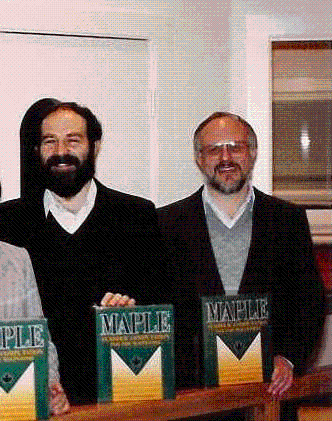
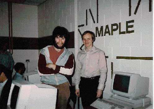
In the beginning (1980) there were two of us: Gaston Gonnet and Keith Geddes 


  • I was on sabbatical at Berkeley during the first half of 1980, hosted by Richard Fatemanstarted writing a textbook on algebraic algorithmswhich eventually got completed (with co-authors) in 1992 :
 

Image 


  • But back to 1980!
 

  • I called a meeting of my CS colleagues at UW in November 1980
 

  • My question: Can we apply for research grant to buy a computer large enough to run MACSYMA?
 

  • The answer (typical of UW): You should build your own system, and (avoiding LISP as an implementation language) try to do much more with fewer computing resources.
 

  • In short, using a BCPL-language (eventually, this meant the C language) we did develop the Maple system which could do more with less!
 

  • It was at this November 1980 meeting where I learned that fellow faculty member, Gaston Gonnet, was also interested in algebraic computation.
 

  • Gaston had already developed a mini-CA system (WAMA -- Waterloo Algebraic Manipulation) during 1979-80, for doing asymptotic analysis calculations related to the analysis of algorithms.
 

  • By the first week of December 1980, Gaston had put together the first running system to which we gave the name "Maple".
 

  • Where does the name "Maple" come from?
    It is just a Canadian name -- after first thinking of acronyms for "Mathematical Programming Language", for example.
 

  • Now I could proceed with my interest in "Algorithms for Computer Algebra" by implementing the algorithms in Maple.


How many Person-Years of R&D for Maple? 


  • Start date is 1 Dec 1980.


  • Of course, we need a Maple calculation to figure out the number of person-years of R&D effort.


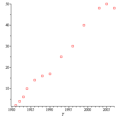
  • Note: The numbers for PersonsPerYear below are fictitious -- but maybe something like this!


> `assign`(PersonsPerYear, [[1981, 2], [1982, 4], [1983, 6], [1984, 10], [1986, 14], [1988, 16], [1990, 17], [1993, 25], [1996, 30], [1999, 40], [2003, 48], [2005, 50], [2007, 48]]); -1
`assign`(PersonsPerYear, [[1981, 2], [1982, 4], [1983, 6], [1984, 10], [1986, 14], [1988, 16], [1990, 17], [1993, 25], [1996, 30], [1999, 40], [2003, 48], [2005, 50], [2007, 48]]); -1
 

> `assign`(DataPlot, plot(PersonsPerYear, Y = 1980 .. 2007, style = point, symbol = BOX, symbolsize = 14)); -1
 

> DataPlot
 

Plot_2d
 

> `assign`(Digits, 4); -1
 

> `assign`(BaseYear, 1980); -1
 

> `assign`(normalize, proc (Y) options operator, arrow; `if`(`::`(Y, name), 'normalize(Y)', `+`(Y, `-`(BaseYear))) end proc)
 

proc (Y) options operator, arrow; `if`(`::`(Y, name), 'normalize(Y)', `+`(Y, `-`(BaseYear))) end proc (3)
 

> `assign`(scaling, proc (l) options operator, arrow; [normalize(l[1]), l[2]] end proc); -1
 

> `assign`(PersonsPerYear, map(scaling, PersonsPerYear))
 

[[1, 2], [2, 4], [3, 6], [4, 10], [6, 14], [8, 16], [10, 17], [13, 25], [16, 30], [19, 40], [23, 48], [25, 50], [27, 48]]
[[1, 2], [2, 4], [3, 6], [4, 10], [6, 14], [8, 16], [10, 17], [13, 25], [16, 30], [19, 40], [23, 48], [25, 50], [27, 48]]
(4)
 

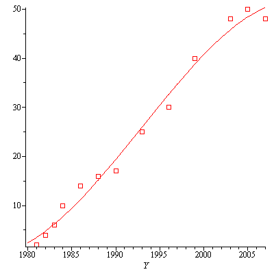
> CurveFitting:-LeastSquares(PersonsPerYear, t, curve = `+`(`*`(a, `*`(`^`(t, 3))), `*`(b, `*`(`^`(t, 2))), `*`(c, `*`(t)), d))
 

`+`(`/`(796348609712, 323896149075), `*`(`/`(630551175617, 647792298150), `*`(t)), `*`(`/`(62732611651, 647792298150), `*`(`^`(t, 2))), `-`(`*`(`/`(806563343, 323896149075), `*`(`^`(t, 3))))) (5)
 

> `assign`(persons, evalf(sort(%)))
 

`+`(`-`(`*`(0.2490e-2, `*`(`^`(t, 3)))), `*`(0.9684e-1, `*`(`^`(t, 2))), `*`(.9734, `*`(t)), 2.459) (6)
 

> `assign`(persons, subs(t = normalize(Y), persons)); -1
 

> `assign`(CurvePlot, plot(persons, Y = 1980 .. 2007)); -1
 

> plots[display]({CurvePlot, DataPlot})
 

Plot_2d
 

> `assign`(PersonYears, int(persons, Y = 1981 .. 2007)); -1
 

> `assign`(PersonYears, evalf(PersonYears))
 

722.8 (7)
 

>


Voila! 


1981-1984: A Few Pictures 


Image 

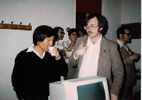
Michael Monagan and Greg Fee 


  • Michael Monagan arrived at UW (from New Zealand) as a graduate student in 1982.
 

  • By the end of the 1980s when we calculated the contributions to Maple code by various authors, Michael was one of the "top three" contributors (Gaston, Keith and Michael) -- in some order (I believe that Michael was ahead of one or both of us).
 

  • Greg Fee and Benton Leong were hired to work on the Maple project about 1981 and remained with the project for many years.


Image 

Benton Leong and Howard Johnson 


Image 

A good view of the "ASCII Maple logo" 


  • Credit for inventing the "ASCII Maple logo" goes to Stephen Watt, who did his PhD degree under my supervision in the early 1980s.


An Aside 

  • There is no truth to the rumour that Stephen got his PhD for inventing the ASCII Maple logo!


Since this is a joint banquet for SNC and PASCO -- 

  • My presentation has not related to the PASCO conference, so let me give some "parallel" relationships.


Stephen Watt's PhD Thesis 

  • Bounded Parallelism in Computer Algebra, 1986
 

  • supervised by me


The 1980 Parallel Maple Question 

  • At discussions with CS colleagues in November 1980, the question arose whether we should consider parallelism in the fundamental design of Maple
    - Morven Gentleman's advice: No, that is a separate research topic
    - I think this was solid advice for our project in 1980


Another relationship to PASCO 

  • Mike Bauer is an Invited Speaker at PASCO on Saturday
 

  • As graduate students at U of T in the early 1970s, Mike and I shared an office!


The 2007 Parallel Maple Question 

More seriously, 

  • although I personally have no project work proceeding on parallelism
 

  • obviously parallelism is an important issue for Maple in this decade


1985-1997: More Pictures 


Image 

Stan Devitt, Stephen Watt, Bruce Char, Benton Leong, Keith Geddes 

(in Linz, Austria for the 1985 Eurocal conference) 


Image 

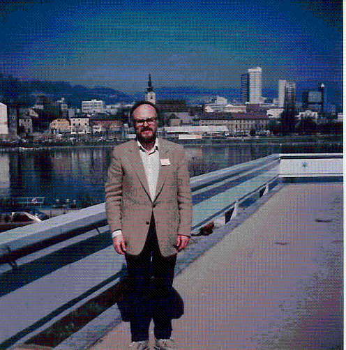
A geeky picture of me in Linz, Austria (1985) 


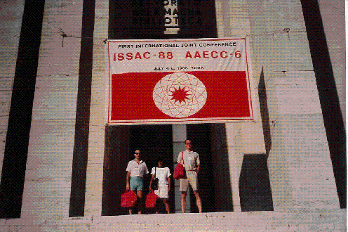
ImageISSAC '88 in Rome -- the first to be named "ISSAC" 
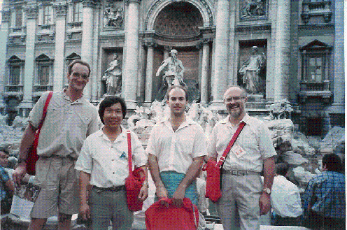


ImageRome 1988 


ImageBruce Char and Mark Mutrie, Maple Retreat 1989 
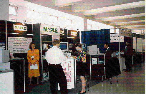


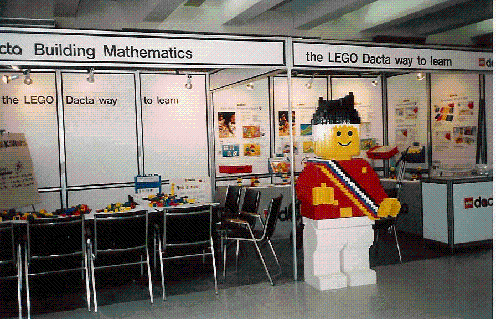
ImageMaple booth, NCTM 1992, Quebec City 


ImageA view of the competition, NCTM 1992, Quebec City 


ImageStephen Watt and I with hosts, Kiev 1993 
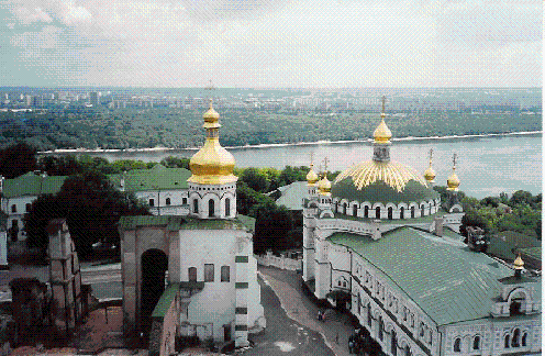


ImageKiev 1993 


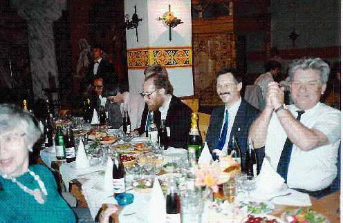
ImageThe vodka banquet, Kiev 1993 


ImageW. Kahan, K. Geddes, D. Jeffrey, G. Labahn, Ha Le, Maple Retreat 1994 
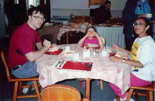


Image 

Rob Corless family, Maple Retreat 1994 


ImageErich Kaltofen with Allan Bonadio and ??, Maple Retreat 1994 
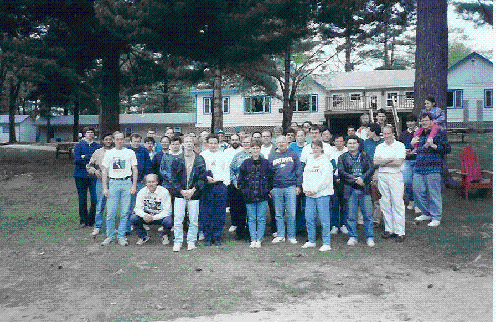


ImageGroup picture, Maple Retreat 1994 


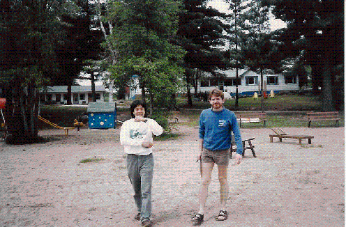
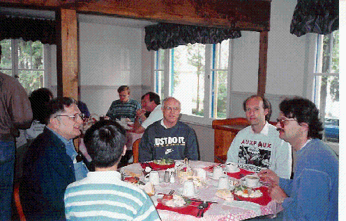
ImageHard at work at the Maple Retreat, Sparrow Lake, Ontario, 1997 


SNC Today 


Conferences/Workshops 

(among others) 


  • SNAP '96, Sophia Antipolis, France, Jul 1996
    (
    Symbolic-Numeric Algebra for Polynomials)


  • SNSC '99, RISC-Linz, Aug 1999
    (
    Symbolic and Numerical Scientific Computation)


  • SNSC '01, RISC-Linz, Sep 2001


  • SNC '05, Xi'an, China, Jul 2005
    (
    Symbolic-Numeric Computation)


  • SNC '07, London, Ontario, Canada, Jul 2007


  • Significant contributions are being presented at these meetings


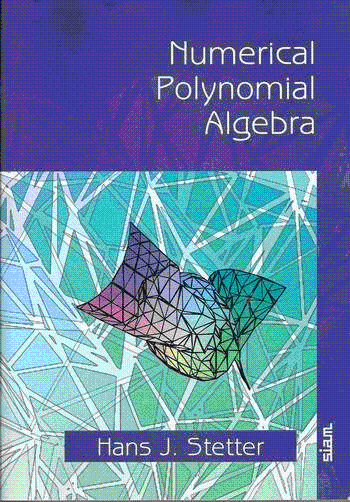
H. J. Stetter 

  • Numerical Polynomial Algebra, 2004.


Image 


ImageHans Stetter, Keith Geddes, Stephen Watt, 2005 


Remarks on Stetter's Book 

As I found in first encounters as a graduate student with Wilkinson's books,
and with the works of Kahan and many others ...


  • Stetter's book can be intimidating at first encounter
    (notation to be mastered, details can be overwhelming).


  • Over time, the fundamental concepts from Wilkinson, Kahan, and others have become "common knowledge" in scientific computing, taught in undergraduate courses.


  • I believe that Stetter has laid a solid foundation for numerical polynomial algebra.


Key concepts 

  • backward error analysis (cf. Wilkinson 1963)
 

  • solving eigenproblems (cf. Wilkinson 1965)
 

  • m-fold clusters of roots (cf. Kahan 1972)
 

  • incorporating these numerical analysis concepts into the context of multivariate polynomial algebra, where the primary tool in the case of exact data is Groebner bases (cf. Buchberger 1965 and later)
 

  • ultimately, pointing the way towards stable numerical algorithms for polynomial algebra


Conclusions 


  • Hopefully over time, the fundamental concepts presented by Stetter (and being further developed by others) will become "common knowledge" in scientific computing.


  • Of course, there is more to Symbolic-Numeric Computation than the topics of Stetter's book!


  • Progress continues on many aspects. As indicated at the outset, I have not attempted to be comprehensive about mentioning the significant contributions to this field.