2-Point Rule
We develop Gaussian quadrature rules for the integral
on the standard interval
. For a general interval of integration
one can perform a simple transformation of variables.
For the 2-point rule, we must choose evaluation points
and corresponding weights
such that the quadrature rule
> |
![`:=`(Q2, `+`(`*`(w1, `*`(f(x1))), `*`(w2, `*`(f(x2)))))](images/GaussQuadrature_6.gif) |
![`+`(`*`(w1, `*`(f(x1))), `*`(w2, `*`(f(x2))))](images/GaussQuadrature_7.gif) |
(1) |
will be exact for integrating polynomials of as high a degree as possible.
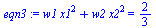
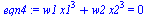
Noting that
forms a basis for all polynomials of degree 3, we set up four (nonlinear) equations in the four unknowns
as follows.
> |
![`:=`(f, proc (x) options operator, arrow; 1 end proc)](images/GaussQuadrature_10.gif) |
![proc (x) options operator, arrow; 1 end proc](images/GaussQuadrature_11.gif) |
(2) |
> |
![`:=`(eqn1, Q2 = int(f(x), x = -1 .. 1))](images/GaussQuadrature_12.gif) |
![`+`(w1, w2) = 2](images/GaussQuadrature_13.gif) |
(3) |
> |
![`:=`(f, proc (x) options operator, arrow; x end proc)](images/GaussQuadrature_14.gif) |
![proc (x) options operator, arrow; x end proc](images/GaussQuadrature_15.gif) |
(4) |
> |
![`:=`(eqn2, Q2 = int(f(x), x = -1 .. 1))](images/GaussQuadrature_16.gif) |
![`+`(`*`(w1, `*`(x1)), `*`(w2, `*`(x2))) = 0](images/GaussQuadrature_17.gif) |
(5) |
> |
![`:=`(f, proc (x) options operator, arrow; `*`(`^`(x, 2)) end proc)](images/GaussQuadrature_18.gif) |
![proc (x) options operator, arrow; `*`(`^`(x, 2)) end proc](images/GaussQuadrature_19.gif) |
(6) |
> |
![`:=`(eqn3, Q2 = int(f(x), x = -1 .. 1))](images/GaussQuadrature_20.gif) |
![`+`(`*`(w1, `*`(`^`(x1, 2))), `*`(w2, `*`(`^`(x2, 2)))) = `/`(2, 3)](images/GaussQuadrature_21.gif) |
(7) |
> |
![`:=`(f, proc (x) options operator, arrow; `*`(`^`(x, 3)) end proc)](images/GaussQuadrature_22.gif) |
![proc (x) options operator, arrow; `*`(`^`(x, 3)) end proc](images/GaussQuadrature_23.gif) |
(8) |
> |
![`:=`(eqn4, Q2 = int(f(x), x = -1 .. 1))](images/GaussQuadrature_24.gif) |
![`+`(`*`(w1, `*`(`^`(x1, 3))), `*`(w2, `*`(`^`(x2, 3)))) = 0](images/GaussQuadrature_25.gif) |
(9) |
> |
![`:=`(_EnvExplicit, true)](images/GaussQuadrature_26.gif) |
![true](images/GaussQuadrature_27.gif) |
(10) |
> |
![solve({eqn1, eqn2, eqn3, eqn4}, {w1, w2, x1, x2})](images/GaussQuadrature_28.gif) |
![{w1 = 1, w2 = 1, x1 = `+`(`*`(`/`(1, 3), `*`(`^`(3, `/`(1, 2))))), x2 = `+`(`-`(`*`(`/`(1, 3), `*`(`^`(3, `/`(1, 2))))))}, {w1 = 1, w2 = 1, x1 = `+`(`-`(`*`(`/`(1, 3), `*`(`^`(3, `/`(1, 2)))))), x2 = ...](images/GaussQuadrature_29.gif) |
(11) |
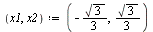
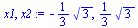
The solution we are interested in is the one with
in order from left to right.
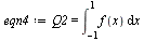
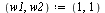
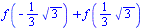
Therefore the 2-point Gaussian quadrature rule for a general function
is as follows.
> |
![`:=`(f, 'f')](images/GaussQuadrature_32.gif) |
![f](images/GaussQuadrature_33.gif) |
(12) |
> |
![`:=`(x1, x2, `+`(`-`(`*`(`/`(1, 3), `*`(sqrt(3))))), `+`(`*`(`/`(1, 3), `*`(sqrt(3)))))](images/GaussQuadrature_34.gif) |
![`+`(`-`(`*`(`/`(1, 3), `*`(`^`(3, `/`(1, 2)))))), `+`(`*`(`/`(1, 3), `*`(`^`(3, `/`(1, 2)))))](images/GaussQuadrature_35.gif) |
(13) |
> |
![`:=`(w1, w2, 1, 1)](images/GaussQuadrature_36.gif) |
![1, 1](images/GaussQuadrature_37.gif) |
(14) |
> |
![Q2](images/GaussQuadrature_38.gif) |
![`+`(f(`+`(`-`(`*`(`/`(1, 3), `*`(`^`(3, `/`(1, 2))))))), f(`+`(`*`(`/`(1, 3), `*`(`^`(3, `/`(1, 2)))))))](images/GaussQuadrature_39.gif) |
(15) |