ScriptC.mw
Parametric Curve Fitting for a Script Letter
Initial Data
The "curve" being used for this example is a script letter C. This illustration is presented using Maple.
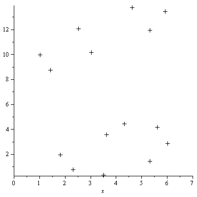
In handwriting, a script C was written on graph paper and then a reasonably small set of  data points was read off from the graph paper. The chosen data points are spaced closer together in regions of high curvature and spaced farther apart in regions of smaller curvature, to achieve the goal of keeping the data set small. See the LinePlot below which shows how the data points are spaced.
In this example, the number of data points is 15.
| > |
 |
| > |
![`:=`(xlist, [1.0, 3.0, 5.3, 5.9, 4.6, 2.5, 1.4, 1.8, 2.3, 3.5, 5.3, 6.0, 5.6, 4.3, 3.6])](images/ScriptC_3.gif) |
![[1.0, 3.0, 5.3, 5.9, 4.6, 2.5, 1.4, 1.8, 2.3, 3.5, 5.3, 6.0, 5.6, 4.3, 3.6]](images/ScriptC_4.gif) |
(1) |
| > |
 |
 |
(2) |
| > |
![`:=`(ylist, [10.0, 10.2, 12.0, 13.5, 13.8, 12.1, 8.8, 2.0, .8, .4, 1.5, 2.9, 4.2, 4.5, 3.6])](images/ScriptC_7.gif) |
![[10.0, 10.2, 12.0, 13.5, 13.8, 12.1, 8.8, 2.0, .8, .4, 1.5, 2.9, 4.2, 4.5, 3.6]](images/ScriptC_8.gif) |
(3) |
| > |
 |
 |
(4) |
| > |
![`:=`(DataPoints, [seq([xlist[i], ylist[i]], i = 1 .. n)])](images/ScriptC_11.gif) |
![[[1.0, 10.0], [3.0, 10.2], [5.3, 12.0], [5.9, 13.5], [4.6, 13.8], [2.5, 12.1], [1.4, 8.8], [1.8, 2.0], [2.3, .8], [3.5, .4], [5.3, 1.5], [6.0, 2.9], [5.6, 4.2], [4.3, 4.5], [3.6, 3.6]]](images/ScriptC_12.gif)
![[[1.0, 10.0], [3.0, 10.2], [5.3, 12.0], [5.9, 13.5], [4.6, 13.8], [2.5, 12.1], [1.4, 8.8], [1.8, 2.0], [2.3, .8], [3.5, .4], [5.3, 1.5], [6.0, 2.9], [5.6, 4.2], [4.3, 4.5], [3.6, 3.6]]](images/ScriptC_13.gif) |
(5) |
The following plot of the data points is not very informative by itself, but when superimposed on future plots it becomes informative.
See the LinePlot below for a better idea of the order of the data points.
| > |
 |
Piecewise-linear Interpolation
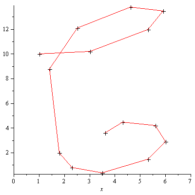
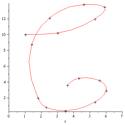
Piecewise-linear (straight-line) interpolation of the data gives an indication of the shape of the letter being represented. For a smooth interpolating curve see the following sections which employ cubic spline interpolation.
| > |
 |
| > |
 |
Cubic Spline Interpolation using Dumb Parameterization
We proceed to do cubic spline interpolation as follows. We parameterize the curve by a parameter  and then compute two cubic spline fits,
  fitting data
  and
and  fitting data
  . The desired curve is then represented by
  as
as  varies over its range of values.
As discussed in class and in the CS 370 Course Notes, the simplest parameterization is achieved by setting  for all
  . However, this leads to a distortion of the curve (illustrated below) due to the fact that in some parts of the curve, successive data points are farther apart than in other parts of the curve. Equally-spaced parameter values fail to reflect this property of the given data.
| > |
![for i to n do `:=`(tlist[i], i) end do; -1](images/ScriptC_31.gif) |
Change  from a Maple table construct to a Maple list construct.
| > |
![`:=`(tlist, [seq(tlist[i], i = 1 .. n)])](images/ScriptC_33.gif) |
![[1, 2, 3, 4, 5, 6, 7, 8, 9, 10, 11, 12, 13, 14, 15]](images/ScriptC_34.gif) |
(6) |
Do cubic spline interpolation to define  and
and  .
.
| > |
 |
| > |
![`:=`(x[cs], Spline(tlist, xlist, t)); -1](images/ScriptC_38.gif) |
| > |
![`:=`(y[cs], Spline(tlist, ylist, t)); -1](images/ScriptC_39.gif) |
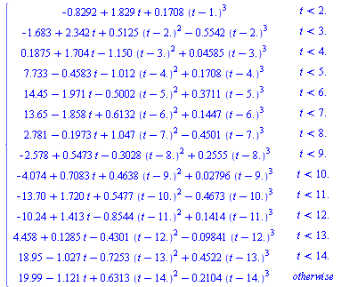
The representation used in Maple for the cubic splines computed by the above commands is a piecewise construct. Below we display the cubic spline  and we round the coefficients to just four significant digits so as to use less space for this display.
| > |
](images/ScriptC_41.gif) |
 |
(7) |
The unapply command appearing below is a Maple construct to transform the given expression into functional form which is useful for subsequent evaluations. For example, if  then the result of the command
  is a function
  such that invoking
  evaluates the expression at the value
  .
.
| > |
![`:=`(x[cs], unapply(x[cs], t)); -1; `:=`(y[cs], unapply(y[cs], t)); -1](images/ScriptC_48.gif) |
The refine Procedure
Corresponding to the Matlab procedure refine presented in the CS 370 Course Notes, we define a Maple procedure to refine the list of evaluation points,  , for the purpose of plotting. In other words, we define a denser set of evaluation points corresponding to the parameter
  so that a plot based on evaluations at the dense set of
  -values will more accurately reflect the cubic spline functions which have been computed.
This procedure will be invoked in the form refine(tlist, refFactor) and the result returned will be a new list of points generated by refining the original list tlist by a factor refFactor.
Plots based on the Dumb Parameterization
First we use a refinement factor of 3 and we display the resulting curve based on evaluating  at 43 points.
| > |
![`:=`(t[ref], refine(tlist, 3))](images/ScriptC_66.gif) |

 |
(8) |
| > |
![`:=`(t[ref], evalf(t[ref]))](images/ScriptC_69.gif) |
| > |
![`:=`(N, nops(t[ref]))](images/ScriptC_75.gif) |
 |
(10) |
| > |
, y[cs](t[ref][i])], i = 1 .. N)]); -1](images/ScriptC_77.gif) |
| > |
 |
| > |
 |
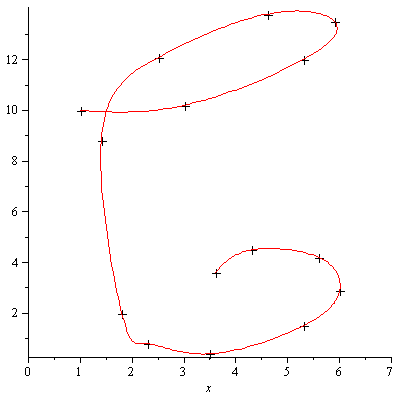
The above plot shows a fairly smooth curve but with some strange kinks.
Let us try a refinement factor of 25 for evaluating the same curve  to see whether the kinks in the above plot are an artifact of not evaluating at a sufficiently dense set of
  -values.
| > |
![`:=`(t[ref], refine(tlist, 25)); -1](images/ScriptC_83.gif) |
| > |
![`:=`(t[ref], evalf(t[ref])); -1](images/ScriptC_84.gif) |
| > |
![`:=`(N, nops(t[ref]))](images/ScriptC_85.gif) |
 |
(11) |
| > |
, y[cs](t[ref][i])], i = 1 .. N)]); -1](images/ScriptC_87.gif) |
| > |
 |
| > |
 |
Although this has achieved some smoothing in parts of the script C, the main kink appearing in the lower part of the curve has not disappeared. This kink is inherent in the particular cubic spline fitting we have done based on the dumb parameterization used above.
Cubic Spline Interpolation using Smart Parameterization
Repeating what was stated above, we parameterize the curve by a parameter  and then compute two cubic spline fits,
  fitting data
  and
and  fitting data
  , where
  are the original 15 data points. The desired curve is then represented by
  as
as  varies over its range of values.
This time we define the parameter values  using a formula based on the distance between successive data points, as discussed in the CS 370 Course Notes.
Recall the original data points.
| > |
 |
![[1.0, 3.0, 5.3, 5.9, 4.6, 2.5, 1.4, 1.8, 2.3, 3.5, 5.3, 6.0, 5.6, 4.3, 3.6]](images/ScriptC_101.gif) |
(12) |
| > |
 |
![[10.0, 10.2, 12.0, 13.5, 13.8, 12.1, 8.8, 2.0, .8, .4, 1.5, 2.9, 4.2, 4.5, 3.6]](images/ScriptC_103.gif) |
(13) |
| > |
 |
 |
(14) |
Define a parameterization based on the distance between successive points.
| > |
![`:=`(tlist[1], 1.0); -1](images/ScriptC_106.gif) |
Change  from a Maple table construct to a Maple list construct.
| > |
![`:=`(tlist, [seq(tlist[i], i = 1 .. n)])](images/ScriptC_111.gif) |
Do cubic spline interpolation to define  and
and  .
.
| > |
![`:=`(x[cs], Spline(tlist, xlist, t)); -1](images/ScriptC_117.gif) |
| > |
![`:=`(y[cs], Spline(tlist, ylist, t)); -1](images/ScriptC_118.gif) |
| > |
![`:=`(x[cs], unapply(x[cs], t)); -1; `:=`(y[cs], unapply(y[cs], t)); -1](images/ScriptC_119.gif) |
First we use a refinement factor of 3 and we display the resulting curve based on evaluating  at 43 points.
| > |
![`:=`(t[ref], refine(tlist, 3)); -1](images/ScriptC_121.gif) |
| > |
![`:=`(t[ref], evalf(t[ref])); -1](images/ScriptC_122.gif) |
| > |
![`:=`(N, nops(t[ref]))](images/ScriptC_123.gif) |
 |
(16) |
| > |
, y[cs](t[ref][i])], i = 1 .. N)]); -1](images/ScriptC_125.gif) |
| > |
 |
| > |
 |
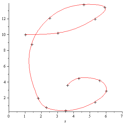
This time we have a somewhat smooth curve and the most significant kink appearing in the previous attempt has disappeared.
Let us try a refinement factor of 25 for evaluating the curve  in order to produce a plot which more accurately reflects the cubic spline fit.
| > |
![`:=`(t[ref], refine(tlist, 25)); -1](images/ScriptC_130.gif) |
| > |
![`:=`(t[ref], evalf(t[ref])); -1](images/ScriptC_131.gif) |
| > |
![`:=`(N, nops(t[ref]))](images/ScriptC_132.gif) |
 |
(17) |
| > |
, y[cs](t[ref][i])], i = 1 .. N)]); -1](images/ScriptC_134.gif) |
| > |
 |
| > |
 |
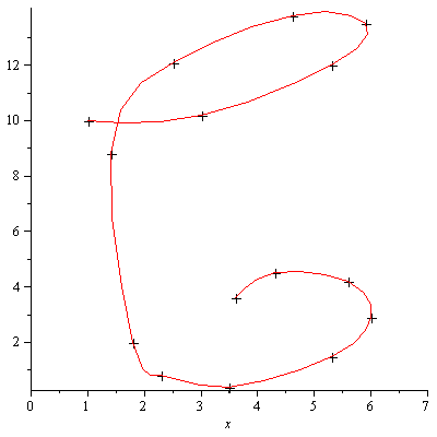
We now have a smooth curve through the given data points. The smart parameterization based on the distance between successive data points avoids the distortion caused by a simple-minded parameterization.
![]() data points was read off from the graph paper. The chosen data points are spaced closer together in regions of high curvature and spaced farther apart in regions of smaller curvature, to achieve the goal of keeping the data set small. See the LinePlot below which shows how the data points are spaced.
data points was read off from the graph paper. The chosen data points are spaced closer together in regions of high curvature and spaced farther apart in regions of smaller curvature, to achieve the goal of keeping the data set small. See the LinePlot below which shows how the data points are spaced. 