PageRank.mw
Example: Google Page Rank
Reference: CS 370 Course Notes, Chapter 5.
The Connectivity Matrix
| > |
 |
| > |
 |
| > |
 |
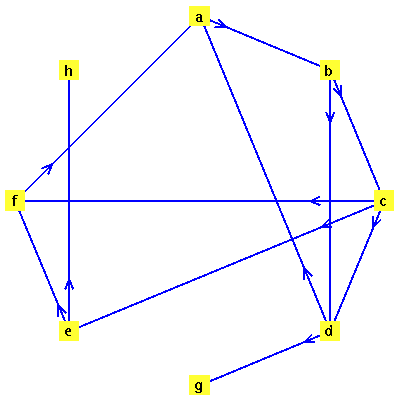
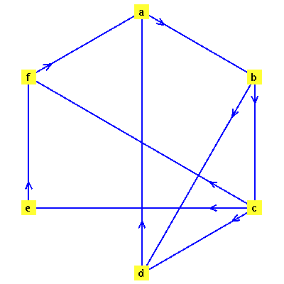
Define a directed graph  with vertices
  and edges
  .
.
| > |
 |
![[a, b, c, d, e, f]](images/PageRank_8.gif) |
(1) |
| > |
 |
![{[a, b], [b, c], [b, d], [c, d], [c, e], [c, f], [d, a], [e, f], [f, a]}](images/PageRank_10.gif) |
(2) |
| > |
 |
![GRAPHLN(directed, unweighted, [a, b, c, d, e, f], Array(%id = 165983624), `GRAPHLN/table/1`, 0)](images/PageRank_12.gif) |
(3) |
| > |
 |
| > |
 |
 |
(4) |
| > |
 |
 |
(5) |
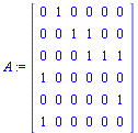
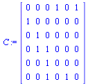
For this application, the connectivity matrix  is the transpose of the graph's adjacency matrix.
| > |
 |
 |
(6) |
Note that the definition of the connectivity matrix  is:
is: 
 if there is a directed arc from node
  to node
  (and 0 otherwise).
The nodes represent web pages and a directed arc from node  to node
  represents the existence of a hyperlink from page
  to page
  .
.
The connectivity matrix  would be very large for the world wide web (there are billions of web pages). However, the matrix is sparse (meaning that there are many zero entries in the matrix).
The  column of
  shows the links on page
  .
.
The outdegree of node  , denoted
  , is the number of arcs leaving node
  .
.
The column sums in  yield the outdegree values:
  (i.e., the
  column sum).
For our example, the outdegrees for nodes  are, respectively,
The Markov Transition Matrix
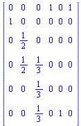
Closely related to the connectivity matrix  , we define a matrix
  of probabilities. We imagine a random web surfer, and
  denotes the probability that the random surfer visits page
  given that he is at page
  . Assuming equal probability of choosing any of the outlinks from page
  , the desired matrix of probabilities is obtained by scaling the connectivity matrix
  by its column sums.
In other words,  if
if  .
.
| > |
 |
| > |
 |
| > |
 |
 |
(7) |
The matrix  is an example of a Markov transition matrix because its elements satisfy
  ≤
≤  and its column sums are all equal to 1.
Dead End Pages and Cycles
In general, the directed graph representing web pages may contain dead end pages, i.e. pages with no outlinks. The corresponding Markov matrix  would have a column of all zeros for any such page. The random surfer would get stuck at such a page. Another problem is cycles: the random surfer might travel endlessly in a cycle of pages such as:
The following modification is for dealing with dead end pages (see Section 5.2.1 of Course Notes):
| > |
 |
 |
(8) |
| > |
 |
 |
(9) |
| > |
 |
 |
(10) |
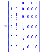
Note that the outer product matrix in this case is a zero matrix (because we have no dead end pages).
| > |
 |
 |
(11) |
To handle cycles (see Section 5.2.2 of Course Notes), we give the random surfer a probability  that he will follow a link from a given page and correspondingly a probability
  that he will teleport to another page (chosen at random) and then continue surfing. Google uses the value
Therefore we update our definition of the Markov transition matrix as follows. As in the Course Notes, we express the formula using the vector  by forming an outer product of
  and its transpose.
| > |
 |
 |
(12) |
| > |
 |
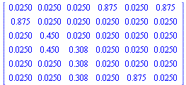
Display  to 3 decimal places.
| > |
 |
 |
(13) |
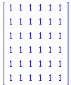
An aside: Note that the outer product operation in this case simply forms a Matrix containing ones.
| > |
 |
 |
(14) |
The matrix  again satisfies the properties of a Markov transition matrix. In particular, note that the column sums are all equal to 1.
| > |
 |
Page Rank Algorithm
A vector  is a probability vector if its entries satisfy
  and
and  . Suppose that
  is a probability vector representing the initial state of the random surfer, and for this initial state use equal probability for each page, as follows.
| > |
 |
 |
(16) |
The  entry
entry  represents the probability that the random surfer is at page
  , and the Markov transition matrix
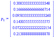
  can be used to calculate the probability vector for the random surfer after one hop, as follows.
| > |
 |
 |
(17) |
Check that this is still a probability vector.
| > |
 |
 |
(18) |
Similarly for the state of the random surfer after two hops, three hops, etc.
| > |
 |
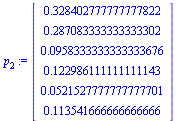 |
(19) |
| > |
 |
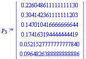 |
(20) |
Check again that this is a probability vector.
| > |
 |
 |
(21) |
Convergence
We wish to obtain a final page ranking as the limit of the above process, because this represents the infinite random hopping of our random surfer.
The question is: Does the above process converge? Theorem 5.7 in the Course Notes proves that the process converges to a unique vector  for any initial probability vector
  . The proof relies on the fact that our Markov transition matrix
  is a positive Markov matrix as defined in the Course Notes.
We can therefore apply the Page Rank Vector Algorithm stated in Section 5.7 of the Course Notes.
| > |
 |
](images/PageRank_114.gif) |
(22) |
Choose a tolerance for the stopping criterion.
(Note that in the actual application to web pages, fewer digits of accuracy would suffice.)
| > |
 |
 |
(23) |
| > |
 |
| > |
 |
 |
(24) |
| > |
 |
](images/PageRank_121.gif) |
(25) |
Look again at the directed graph we are modelling and compare the page rankings specified by  .
.
| > |
 |
| > |
 |
Eigenvector Formulation
The above method is actually performing what is known as the power method for finding the eigenvector of the matrix  corresponding to its largest eigenvalue.
To see this, note that if we had converged to the limiting vector  then we would have:
  . The definition of an eigenvalue λ and its corresponding eigenvector
  is that
  . Therefore, we are computing the eigenvector
  corresponding to the eigenvalue
  .
.
Note: The eigenvalues of a matrix  are the zeros of the characteristic polynomial
  where
where  denotes the identity matrix. The eigenvectors corresponding to an eigenvalue
  are the solutions of the singular linear system
  which we know is a singular system because the determinant is zero.
This all works because, as discussed in the Course Notes, for a positive Markov matrix  the largest eigenvalue is
  and there is only one eigenvector corresponding to this eigenvalue.
To check these facts, let us compute the eigenvalues and eigenvectors of the matrix  .
.
First, for clarification, let us compute the eigenvalues via the characteristic polynomial.
| > |
 |
| > |
 |

 |
(26) |
| > |
 |

 |
(27) |
| > |
 |
![[1.000000001, .6266196805, .4707151655, 0.1149411552e-7, .4707151655, .6266196805]](images/PageRank_149.gif) |
(28) |
Note that the eigenvalue largest in magnitude is  .
.
We can use the command Eigenvectors in Maple to compute the eigenvalues and eigenvectors.
| > |
 |
| > |
 |
 |
(29) |
| > |
 |
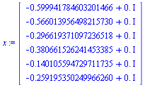 |
(30) |
An eigenvector is unique only up to a scaling factor. The eigenvector we are computing in our Page Rank Algorithm has all entries positive and its 1-norm is equal to 1 (i.e., the sum of the entries is equal to 1).
Scale the eigenvector  by first making the entries positive, then divide by the 1-norm of
  .
.
| > |
 |
| > |
 |
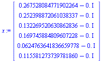 |
(31) |
Check that this normalized eigenvector  corresponds to the vector
  computed by our Page Rank Algorithm.
| > |
 |
 |
(32) |
| > |
 |
](images/PageRank_166.gif) |
(33) |
| > |
 |
](images/PageRank_168.gif) |
(34) |
We see that  corresponds to the normalized eigenvector
  to within the accuracy tolerance
  used in our Page Rank Algorithm.
Example 2: A Graph with Dead Ends
Consider a second example, this time a case where there are dead end pages. We add two dead end pages to the previous example.
| > |
 |
| > |
 |
![[a, b, c, d, e, f, g, h]](images/PageRank_174.gif) |
(35) |
| > |
 |
![{[a, b], [b, c], [b, d], [c, d], [c, e], [c, f], [d, a], [e, f], [f, a], [d, g], [e, h]}](images/PageRank_176.gif) |
(36) |
| > |
 |
![GRAPHLN(directed, unweighted, [a, b, c, d, e, f, g, h], Array(%id = 181551868), `GRAPHLN/table/4`, 0)](images/PageRank_178.gif) |
(37) |
| > |
 |
| > |
 |
 |
(38) |
| > |
 |
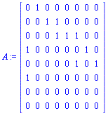 |
(39) |
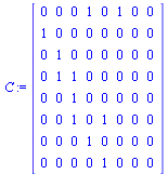
The connectivity matrix  is the transpose of the graph's adjacency matrix.
| > |
 |
 |
(40) |
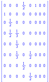
Form the probability matrix  as before.
| > |
 |
| > |
 |
 |
(41) |
The Markov Transition Matrix
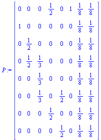
Adjust the matrix  to deal with dead end pages as discussed in the previous example.
| > |
 |
 |
(42) |
| > |
 |
 |
(43) |
| > |
 |
 |
(44) |
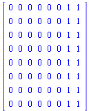
Note that the outer product matrix has ones in the columns that were previously zero, and then we multiply by the probability  (equal probability of teleporting to any of the pages).
| > |
 |
 |
(45) |
As before, avoid the possibility of cycles by using a probability  of teleporting to a random page.
| > |
 |
 |
(46) |
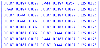
| > |
 |
Display  to 3 decimal places.
| > |
 |
 |
(47) |
The matrix  must satisfy the properties of a Markov transition matrix. In particular, the column sums must be all equal to 1.
| > |
 |
Page Rank Algorithm
| > |
 |
 |
(49) |
| > |
 |
 |
(50) |
| > |
 |
 |
(51) |
| > |
 |
 |
(52) |
| > |
 |
| > |
 |
 |
(53) |
| > |
 |
](images/PageRank_235.gif) |
(54) |
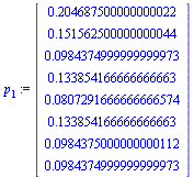
Look again at the directed graph we are modelling and compare the page rankings specified by  .
.
| > |
 |
| > |
 |
![]() with vertices
with vertices ![]() and edges
and edges ![]() .
. 

![]() is the transpose of the graph's adjacency matrix.
is the transpose of the graph's adjacency matrix. 
![]() is:
is: ![]()
![]() if there is a directed arc from node
if there is a directed arc from node ![]() to node
to node ![]() (and 0 otherwise).
(and 0 otherwise). ![]() to node
to node ![]() represents the existence of a hyperlink from page
represents the existence of a hyperlink from page ![]() to page
to page ![]() .
. ![]() would be very large for the world wide web (there are billions of web pages). However, the matrix is sparse (meaning that there are many zero entries in the matrix).
would be very large for the world wide web (there are billions of web pages). However, the matrix is sparse (meaning that there are many zero entries in the matrix). ![]() column of
column of ![]() shows the links on page
shows the links on page ![]() .
. ![]() , denoted
, denoted ![]() , is the number of arcs leaving node
, is the number of arcs leaving node ![]() .
. ![]() yield the outdegree values:
yield the outdegree values: ![]() (i.e., the
(i.e., the ![]() column sum).
column sum). ![]() are, respectively,
are, respectively, ![]()


](images/PageRank_121.gif)


](images/PageRank_166.gif)
](images/PageRank_168.gif)


](images/PageRank_235.gif)
