Conversion to a First-Order System
If a given system of ordinary differential equations (ODEs) involves derivatives higher than first order, then in order to apply a numerical solution method the ODEs must be converted to a system of first-order ODEs.
In Maple, the conversion of higher-order ODEs to a first-order system is handled automatically when a numerical solution is requested. In Matlab or any other purely numerical computation environment, the conversion to a first-order system must be done manually by the user.
Example 1: A 2nd-order ODE
Consider the following initial-value problem (IVP) appearing in Example 9.3 of the CS 370 Course Notes.
| > |
 |
| > |
 |
 |
(1) |
with initial conditions
| > |
 |
![y(0) = y[0], (D(y))(0) = 3](images/ODE_Systems_5.gif) |
(2) |
This can be converted to a first-order system as follows. Introduce a new set of dependent variables:
| > |
 |
 = y(t)](images/ODE_Systems_7.gif) |
 = diff(y(t), t)](images/ODE_Systems_8.gif) |
(3) |
In terms of the new functions  the original
  -order ODE becomes the following first-order system, where the last equation involves isolating the highest-order derivative on the left hand side of the original equation.
| > |
 |
, t) = y[2](t)](images/ODE_Systems_12.gif) |
, t) = `+`(`*`(t, `*`(y[2](t))), `-`(`*`(a, `*`(y[1](t)))), sin(t))](images/ODE_Systems_13.gif) |
(4) |
with initial conditions
| > |
 |
 = y[0], y[2](0) = 3](images/ODE_Systems_15.gif) |
(5) |
This now takes the form of a standard first-order system:
| > |
 |
 |
 |
(6) |
where  is a vector of dimension 2 and
  is a vector function of dimension 2 taking as arguments
  and the vector
  . Specifically,
| > |
 |
| > |
 |
 |
(7) |
| > |
 |
| > |
 |
 |
(8) |
The initial conditions are specified by the vector  :
:
| > |
 |
| > |
 |
 |
(9) |
Example 2: A 4th-order ODE
| > |
 |
| > |
 |
 |
(10) |
with initial conditions
| > |
 |
 |
(11) |
This can be converted to a first-order system as follows. Introduce a new set of dependent variables:
| > |
 |
In terms of the new functions  the original
  -order ODE becomes the following first-order system, where the last equation involves isolating the highest-order derivative on the left hand side of the original equation.
| > |

 |
with initial conditions
| > |
 |
 = 0, y[2](1) = .5, y[3](1) = .1, y[4](1) = 0](images/ODE_Systems_52.gif) |
(14) |
This now takes the form of a standard first-order system:
| > |
 |
 |
 |
(15) |
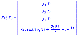
where  is a vector of dimension 4 and
  is a vector function of dimension 4 taking as arguments
  and the vector
  . Specifically,
| > |
 |
| > |
 |
 |
(16) |
| > |
 |
| > |
 |
 |
(17) |
The initial conditions are specified by the vector  :
:
| > |
 |
| > |
 |
 |
(18) |
Example 3: Novelty Golf Driving Range
Consider the following system of ODEs introduced in the CS 370 Course Notes (section 8.2) for the Novelty Golf Driving Range.
| > |
 |
| > |
 |
![diff(x(t), t) = V[x]](images/ODE_Systems_72.gif) |
 |
(19) |
with initial conditions
| > |
 |
![x(0) = 0, y(0) = 0, (D(y))(0) = V[y]](images/ODE_Systems_75.gif) |
(20) |
This can be converted to a first-order system as follows. Introduce a new set of dependent variables:
| > |
 |
In terms of the new functions  the original system of ODEs becomes the following first-order system.
| > |
 |
with initial conditions
| > |
 |
 = 0, y[2](0) = 0, y[3](0) = V[y]](images/ODE_Systems_86.gif) |
(23) |
This now takes the form of a standard first-order system:
| > |
 |
 |
 |
(24) |
where  is a vector of dimension 3 and
  is a vector function of dimension 3 taking as arguments
  and the vector
  . Specifically,
| > |
 |
| > |
 |
 |
(25) |
| > |
 |
| > |
 |
 |
(26) |
The initial conditions are specified by the vector  :
:
| > |
 |
| > |
 |
 |
(27) |
Forward Euler Method for a System
The Forward Euler Method we developed for a single first-order ODE is easily adapted for solving a system of first-order ODEs.
| > |
 |
Let us apply this procedure to solve the IVP of Example 1 above.
Define the system dynamics function.
| > |
 |
| > |
 |
 |
(28) |
Values must be specified for the two parameters  and
and  .
.
| > |
 |
 |
 |
(29) |
The vector  of initial conditions is
| > |
 |
 |
(30) |
Specify the range of integration and the stepsize  .
.
| > |
 |
 |
(31) |
| > |
 |
 |
(32) |
| > |
 |
Compare with the solution obtained by Maple for the original  -order system.
| > |
 |
| > |
 |
 |
(34) |
| > |
 |
 |
(35) |
| > |
 |
 |
(36) |
| > |
 |
![]() the original
the original ![]() -order ODE becomes the following first-order system, where the last equation involves isolating the highest-order derivative on the left hand side of the original equation.
-order ODE becomes the following first-order system, where the last equation involves isolating the highest-order derivative on the left hand side of the original equation. ![]() is a vector of dimension 2 and
is a vector of dimension 2 and ![]() is a vector function of dimension 2 taking as arguments
is a vector function of dimension 2 taking as arguments ![]() and the vector
and the vector ![]() . Specifically,
. Specifically, ![]() :
: ![]() the original
the original ![]() -order ODE becomes the following first-order system, where the last equation involves isolating the highest-order derivative on the left hand side of the original equation.
-order ODE becomes the following first-order system, where the last equation involves isolating the highest-order derivative on the left hand side of the original equation. ![]() is a vector of dimension 4 and
is a vector of dimension 4 and ![]() is a vector function of dimension 4 taking as arguments
is a vector function of dimension 4 taking as arguments ![]() and the vector
and the vector ![]() . Specifically,
. Specifically, 

![]() :
: 
![]() the original system of ODEs becomes the following first-order system.
the original system of ODEs becomes the following first-order system. ![]() is a vector of dimension 3 and
is a vector of dimension 3 and ![]() is a vector function of dimension 3 taking as arguments
is a vector function of dimension 3 taking as arguments ![]() and the vector
and the vector ![]() . Specifically,
. Specifically, 

![]() :
: 