EulerMethods.mw
Numerical Solution of IVPs
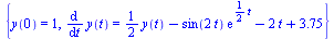
Define an Initial Value Problem
| > |
 |
| > |
 |
 |
(1) |
| > |
 |
| > |
 |
| > |
 |
 |
(2) |
The solution is to be computed for the range  and define
  .
.
| > |
 |
 |
(3) |
| > |
 |
 |
(4) |
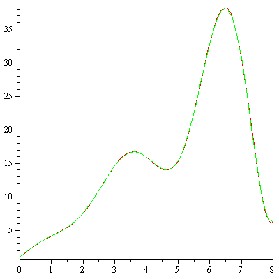
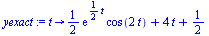
For this example, the exact solution can be expressed in closed form. This will allow us to compare our numerical solution with the exact result.
| > |
 |
 |
(5) |
| > |
 |
 |
(6) |
| > |
 |
| > |
 |
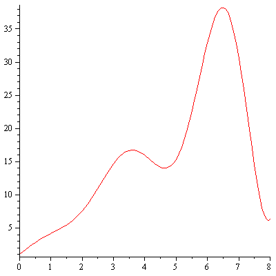
Maple's default numerical solution
| > |
 |
 |
(7) |
| > |
 |
 |
(8) |
| > |
 |
Compare with the true solution at  .
.
| > |
 |
 |
(10) |
| > |
 |
| > |
 |
Forward Euler Method
The Forward Euler Method can be derived from the Taylor series expansion of  with local truncation error
  .
.
This is a method of order 1 because the global truncation error after  steps where
  is:
is:  .
.
| > |
 |
![y(`+`(t[n], h)) = series(`+`(y(t[n]), `*`((D(y))(t[n]), `*`(h)))+O(`^`(h, 2)),h,2)](images/EulerMethods_55.gif) |
(11) |
Here  is the differentiation operator so
  .
.
The resulting formula for the numerical method is:  where
where  .
.
First solve the IVP for the range  with step size
  .
.
| > |
 |
 |
(12) |
| > |
 |
 |
(13) |
| > |
 |
Compare the computed solution with the true solution at  .
.
| > |
 |
 |
(14) |
| > |
 |
 |
(15) |
| > |
 |
 |
(16) |
| > |
 |
 |
(17) |
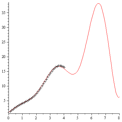
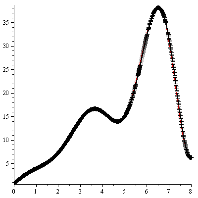
Plot the numerical values and the curve of the true solution.
| > |
 |
| > |
 |
| > |
 |
| > |
 |
Note that the numerical values are off the curve near  .
.
Next, solve the IVP for the range  with the same step size
  .
.
| > |
 |
 |
(18) |
| > |
 |
 |
(19) |
| > |
 |
Compare the computed solution with the true solution at  .
.
| > |
 |
 |
(20) |
| > |
 |
 |
(21) |
| > |
 |
 |
(22) |
| > |
 |
 |
(23) |
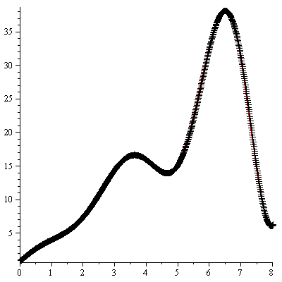
Plot the numerical values and the curve of the true solution.
| > |
 |
| > |
 |
| > |
 |
| > |
 |
The numerical solution is not very accurate.
This time, solve the IVP for the range  with a smaller step size
  .
.
| > |
 |
 |
(24) |
| > |
 |
 |
(25) |
| > |
 |
Compare the computed solution with the true solution at  .
.
| > |
 |
 |
(26) |
| > |
 |
 |
(27) |
| > |
 |
 |
(28) |
| > |
 |
 |
(29) |
Plot the numerical values and the curve of the true solution.
| > |
 |
| > |
 |
| > |
 |
| > |
 |
Modified Euler Method
For the Modified Euler Method, we start with one more term in the Taylor series expansion of  . This time the local truncation error is
  .
.
This is a method of order 2 because the global truncation error after  steps where
  is:
is: 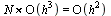 .
.
| > |
 |
| > |
 |
| > |
 |
![y(`+`(t[n], h)) = series(`+`(y(t[n]), `*`((D(y))(t[n]), `*`(h)), `*`(`*`(`/`(1, 2), `*`(((`@@`(D, 2))(y))(t[n]))), `*`(`^`(h, 2))))+O(`^`(h, 3)),h,3)](images/EulerMethods_162.gif) |
(30) |
With  and
and 
we have the following potential numerical formula: 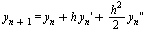 .
.
While we know that, as before,  we will have to approximate
  in some manner.
We will use the divided difference approximation: 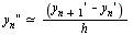 .
.
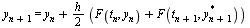
This leads to the following formula for the numerical method:
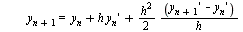
or, collecting terms
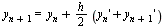 .
.
From the IVP we know that  so we have developed the following implicit formula for
  :
:
| > |
 |
![y[`+`(n, 1)] = `+`(y[n], `*`(`/`(1, 2), `*`(h, `*`(`+`(F(t[n], y[n]), F(t[`+`(n, 1)], y[`+`(n, 1)]))))))](images/EulerMethods_174.gif) |
(31) |
For the Modified Euler Method, we transform this into an explicit formula for  via a two-step method.
Apply the Forward Euler Method to compute a first approximation for  :
:
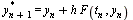
and then use this value in formula 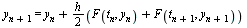 to get
 .
.
The Modified Euler Method is one member of a class of methods known as Runge-Kutta methods.
Specifically, this is a Runge-Kutta method of order 2.
The formulas are often written in the following form.
| > |
 |
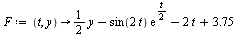
Restore the definition of  for our particular IVP.
| > |
 |
 |
(33) |
Solve the IVP for the range  with step size
  .
.
| > |
 |
 |
(34) |
| > |
 |
 |
(35) |
| > |
 |
Compare the computed solution with the true solution at  .
.
| > |
 |
 |
(36) |
| > |
 |
 |
(37) |
| > |
 |
 |
(38) |
| > |
 |
 |
(39) |
The numerical value at  is more accurate than before.
Also, note that the value at the point  is accurate to 3 significant figures this time.
| > |
 |
 |
(40) |
| > |
 |
 |
(41) |
| > |
 |
 |
(42) |
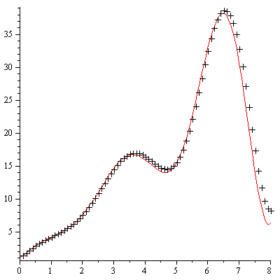
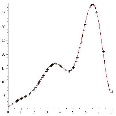
Plot the numerical values and the curve of the true solution.
| > |
 |
| > |
 |
| > |
 |
| > |
 |
The computed solution follows the curve of the true solution much better with this method.
Now solve the IVP for the range  with a smaller step size
  .
.
| > |
 |
 |
(43) |
| > |
 |
 |
(44) |
| > |
 |
Compare the computed solution with the true solution at  .
.
| > |
 |
 |
(45) |
| > |
 |
 |
(46) |
| > |
 |
 |
(47) |
| > |
 |
 |
(48) |
Plot the numerical values and the curve of the true solution.
| > |
 |
| > |
 |
| > |
 |
| > |
 |
Test Order of Accuracy: ForwardEuler
| > |
 |
 |
(49) |
| > |
 |
 |
(50) |
| > |
 |
 |
(51) |
| > |
 |
| > |
 |
 |
(52) |
| > |
 |
 |
(53) |
| > |
 |
](images/EulerMethods_289.gif) |
(54) |
Compute successive ratios
| > |
 |
The ratio is approximately  .
.
Conclusion: Since 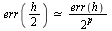 with
with  we conclude that ForwardEuler is of order 1.
Test Order of Accuracy: ModifiedEuler
| > |
 |
 |
(56) |
| > |
 |
 |
(57) |
| > |
 |
 |
(58) |
| > |
 |
| > |
 |
 |
(59) |
| > |
 |
 |
(60) |
| > |
 |
](images/EulerMethods_321.gif) |
(61) |
Compute successive ratios
| > |
 |
The ratio is approximately  .
.
Conclusion: Since  with
with  we conclude that ModifiedEuler is of order 2.
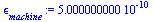
Effects of Roundoff Error
Note that the last couple of values of  are contaminated by roundoff errors in computing the numerical solution, so they are meaningless.
In fact, recall the number of steps used for computing the numerical solution that determined  :
:
| > |
 |
 |
(63) |
We know from our study of "Floating Point Arithmetic" that adding  numbers can incur a relative error of approximately
  . (This is in the "best case" where we are adding numbers all of the same sign.)
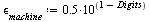
We are computing with Maple's default number of Digits and therefore  is as follows:
| > |
 |
 |
(64) |
| > |
 |
 |
(65) |
Therefore, the accumulated roundoff error when computing the numerical method with  steps can be expected to be approximately:
| > |
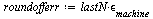 |
 |
(66) |
I.e., 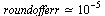 . Note that it is precisely at this level of accuracy in the values of
  that halving
  fails to yield improved accuracy.
| > |
 |
](images/EulerMethods_353.gif) |
(67) |