6. Reductions
We saw two examples of reductions in the last lecture. Both were used to show that a particular language (\(A_{TM}^\epsilon\) and \(BB\), respectively) is undecidable. But the reductions themselves were quite different from each other. Indeed, they are representative examples of two distinct types of reductions: mapping reductions and Turing reductions. These two types of reductions both can be used to prove undecidability of languages. And, as we will see, they can also be used to study questions of computability that go even beyond decidability.
Mapping Reductions
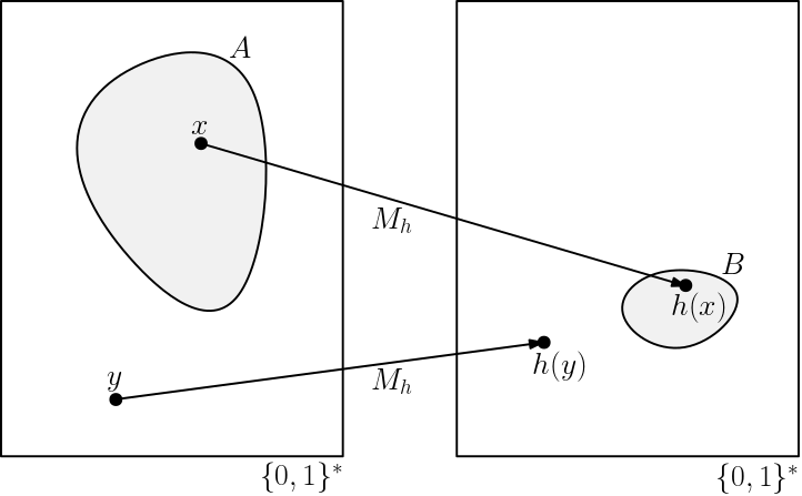
Fix any two languages \(A, B \subseteq \{0,1\}^*\). There is a mapping reduction from \(A\) to \(B\), denoted
\[A \le_m B\]if there is a function \(h \colon \{0,1\}^* \to \{0,1\}^*\) that satisfies two conditions:
- Every \(x \in \{0,1\}^*\) satisfies \(x \in A \Leftrightarrow h(x) \in B\).
- There is a Turing machine \(M_h\) that on every input \(x \in \{0,1\}^*\) halts with \(h(x)\) on the tape.
(We say that the machine \(M_h\) computes the function \(h\) when it satisfies the second condition, and that a function \(h\) is computable when there is a machine \(M_h\) that computes it.)
The notion of a mapping reduction can be represented visually as follows:
Note that the mapping \(h\) does not have to be one-to-one or onto. In the most extreme case, it is even possible for \(h\) to map each \(x \in A\) to the same element \(y \in B\) and to map all \(x' \notin A\) to a single \(y' \notin B\).
The notation \(A \le_m B\) suggests that when there is a mapping reduction from \(A\) to \(B\), \(A\) is “no harder” than \(B\). This is indeed the case when we consider decidability.
Theorem. For any two languages \(A, B \subseteq \{0,1\}^*\) that satisfy \(A \le_m B\),
- If \(B\) is decidable, then so is \(A\); and
- If \(A\) is undecidable, then so is \(B\).
Proof. The two conclusions are contrapositives of each other, so we only need to prove the first one.
Let \(h\) be a mapping that establishes the reduction \(A \le_m B\) and \(M_h\) be a Turing machine that computes \(h\). Let \(M_B\) be a Turing machine that decides \(B\). Define \(M_A\) to be the Turing machine obtained by concatenating \(M_h\) and \(M_B\). Then on any input \(x\),
- \(M_h\) halts with \(h(x)\) on the tape, then
- \(M_B\) accepts if \(h(x) \in B\) and rejects otherwise.
Therefore, \(M_A\) always halts, and it accepts \(x\) if and only if \(h(x) \in B\). But by the first condition on \(h\), this is the case if and only if \(x \in A\), so \(M_A\) decides \(A\).
The mapping reduction \(A \le_m B\) also shows that \(A\) is “no harder” than \(B\) when we consider recognizability instead of decidability. Recall that a language \(L\) is recognizable if there is a Turing machine \(M\) such that
\[L = L(M) := \{ x \in \{0,1\}^* : M \mbox{ accepts } x \}.\](In this definition, the machine \(M\) can either reject or run forever on inputs that are not in the language.) Then essentially the same argument as in the last proof also establishes the following result.
Theorem. For any two languages \(A, B \subseteq \{0,1\}^*\) that satisfy \(A \le_m B\),
- If \(B\) is recognizable, then so is \(A\); and
- If \(A\) is unrecognizable, then so is \(B\).
Unrecognizable Languages
Before we can use mapping reductions to prove unrecognizability, we first need to identify an unrecognizable language. We can find one by first asking some basic questions about the set of recognizable languages.
Every decidable language is recognizable, as we can see directly from the definitions. Are there also some undecidable languages that are recognizable?
Proposition 5. The undecidable language \(A_{TM}\) is recognizable.
Proof. Consider the Universal Turing Machine \(U\). On input \(\left< M \right> x\), it simulates \(M\) on \(x\) and, in particular, accepts if and only if \(M\) accepts \(x\). Therefore, \(U\) recognizes \(A_{TM}\).
Is it also possible for a language \(L\) and its complement \(\overline{L} = \{0,1\}^* \setminus L\) to both be recognizable and yet have \(L\) still be undecidable?
Theorem 6. If a language \(L\) and its complement \(\overline{L} = \{0,1\}^* \setminus L\) are both recognizable, then \(L\) and \(\overline{L}\) are both decidable.
Proof. Assume that \(T_1\) and \(T_2\) recognize \(L\) and \(\overline{L}\), respectively.
Let \(M\) be a Turing machine that simulates both \(T_1\) and \(T_2\) in parallel. Specifically, it dedicates separate portions of the tape for the simulation of both \(T_1\) and \(T_2\) and interleaves their simulations by performing one step of computation of each of them at a time. The simulation is completed when either \(T_1\) or \(T_2\) accepts. If \(T_1\) is the machine that accepts, \(M\) also accepts. Otherwise, if \(T_2\) accepts then \(M\) rejects.
When \(x \in L\), then \(T_1\) is guaranteed to accept \(x\) after a finite number of steps, and \(T_2\) is guaranteed not to accept, so \(M\) correctly accepts \(x\). Similarly, when \(x \in \overline{L}\) then \(T_2\) is guaranteed to accept after a finite number of steps and \(T_1\) will not accept so \(M\) correctly rejects \(x\). Therefore, \(M\) decides \(L\), and the machine \(M'\) obtained by switching the accept and reject labels in \(M\) decides \(\overline{L}\).
We can use this result to obtain an explicit language that is not recognizable:
Corollary. The language \(\overline{A_{TM}}\) is unrecognizable.
Proof. We have already seen that \(A_{TM}\) is recognizable. If \(\overline{A_{TM}}\) was also recognizable, then by Theorem 6 the language \(A_{TM}\) would be decidable, which we already know is false.
We can now use mapping reductions to establish the unrecognizability of other languages.
Theorem. The language \(\mathsf{Empty}_{TM}\) is unrecognizable.
Proof. We show that \(\overline{A}_{TM} \le_m \mathsf{Empty}_{TM}\). Consider the function \(h\) that maps the string \(\left< M \right> x\) to the string \(\left< M'_x \right>\) where \(M'_x\) is the TM that on input \(y\):
- Checks if \(y = x\); if not, it rejects.
- If \(y = x\), it runs \(M\) on \(x\).
The function \(h\) can be computed by a Turing machine. And the language of \(M'_x\) is either the singleton set \(\{x\}\) or the empty set, depending on whether \(M\) accepts \(x\) or not. So \(L(M'_x) = \emptyset\) if and only if \(M\) does not accept \(x\). In other words, \(h(\left< M \right> x) = \left< M'_x \right> \in \mathsf{Empty}_{TM}\) if and only if \(\left< M \right> x \in \overline{A}_{TM}\).
Turing Reductions
Another way that we can show a language \(A\) is “no harder” than some other language \(B\) is to show that if we can (somehow) decide \(B\), we can construct a Turing machine that also decides \(A\). This notion can be made precise with the concept of oracle Turing machines.
An oracle Turing machine is a slight extension of the standard model of Turing machines that we have considered so far where we also add a second special tape that we call the oracle tape. The Turing machine can read and write to the oracle tape just as it does on the regular tape. And it also has a special operation it can perform to query the oracle: when it performs this operation, the contents \(x\) of the oracle tape is replaced with either \(0\) or \(1\). An oracle Turing machine can query the oracle as often as it likes, and otherwise behaves exactly the same as regular Turing machines.
Note that we have not defined how the oracle answers the queries made by the oracle Turing machine. By default, it always answers each query with \(0\); in this case, we can see that oracle Turing machines are equivalent to standard Turing machines. (I.e., the oracle tape does not add any additional power to Turing machines if we use this default behaviour.) But we can also provide a non-trivial oracle to an oracle Turing machine by specifying a language \(A \subseteq \{0,1\}^*\). When we do so, the query \(x\) to the oracle returns \(1\) when \(x \in A\) and \(0\) when \(x \notin A\). We write \(M^A\) to denote the oracle Turing machine \(M\) with oracle access to \(A\).
We can use oracle Turing machines to define our second type of reduction. There is a Turing reduction from \(A\) to \(B\), denoted
\[A \le_T B\]when there is an oracle Turing machine \(M\) such that the machine \(M^B\) with oracle access to \(B\) decides \(A\).
Turing reducibility is a weaker notion than mapping reducibility, in the sense that every pair of languages that satisfies \(A \le_m B\) also satisfies \(A \le_T B\), but the other direction does not always hold. Turing reducibility also captures the notion of a relation of hardness of languages in terms of decidability.
Theorem. For any two languages \(A, B \subseteq \{0,1\}^*\) that satisfy \(A \le_T B\),
- If \(B\) is decidable, then so is \(A\); and
- If \(A\) is undecidable, then so is \(B\).
There exists recognizable \(A\) and unrecognizable \(B\) for which \(A \le_T B\), so Turing reducibility cannot be used to establish unrecognizability of languages. Nonetheless, as we see below, the notion of oracle Turing machines that we used to define Turing reductions can be used to examine other interesting extensions of the set of all decidable languages.
Turing Degrees
Here’s a natural question worth examining: is \(A_{TM}\) the “only” barrier to decidability? Or, more precisely, if I was somehow given a (magical?) device that could always tell me if a Turing machine halts on a given input, could I use it to decide every other language?
We can formalize (the complement of) the last question using oracle Turing machines: are there languages that cannot be computed by \(M^{A_{TM}}\) for any oracle Turing machine \(M\)? We will call such languages undecidable relative to \(A_{TM}\). Since there are uncountably many languages and only countably many oracle Turing machines, we do know that there are languages which are undecidable relative to \(A_{TM}\). We can also give an example of such a function:
Theorem. The language
\[A'_{TM} = \{ \left< M \right> x : M \mbox{ is an oracle TM and } M^{A_{TM}} \mbox{ accepts } x\}\]is undecidable relative to \(A_{TM}\).
Proof. Assume on the contrary that \(T^{A_{TM}}\) decides \(A'_{TM}\). Let us construct a TM \(D\) using the Recursion Theorem for oracle Turing machines. (Exercise: see how the proof of the Recursion Theorem holds essentially as-is if we replace standard TMs with oracle TMs.) On input \(x\), \(D\):
- Gets its description \(\left< D \right>\).
- Runs \(T\) on \(\left< D \right> x\).
- If \(T\) accepts, reject; otherwise if \(T\) rejects, accept.
The key observation here is that when we run \(T\) in step 2, we do it with \(D\)’s oracle tape. So any oracle passed to \(D\) will be used by \(T\). And this means that \(D^{A_{TM}}\) calls \(T^{A_{TM}}\) in the second step, but then \(D^{A_{TM}}\) accepts \(x\) if and only if \(T^{A_{TM}}\) rejects \(\left< D \right> x\), contradicting the assumption that \(T^{A_{TM}}\) decides \(A'_{TM}\).
We can now ask about the existence of a language that is undecidable relative to \(A'_{TM}\). With the same argument as above, we find that
\[A''_{TM} = \{ \left< M \right> x : M \mbox{ is an oracle TM and } M^{A'_{TM}} \mbox{ accepts } x\}\]is one such language. And continuing this process, we can find an infinite sequence of languages, each “even more” undecidable than the last. In fact, there is a lot more that we can say about the various classes of languages that we obtain by measuring relative undecidability. Doing so leads to the study of Turing degrees and a number of other research directions in computability theory. But instead of going in this direction, starting next lecture we will instead see how we can further partition the set of decidable languages into smaller classes using complexity theory.