2. Turing Machines

We saw in the last lecture that for every fixed machine, there exists a language that cannot be computed by algorithms for that specific machine. Our goal today is to strengthen this result to identify an explicit language that cannot be computed by algorithms over any machine model.

That is where Turing machines come in. The magic of this model of computation is that it satisfies what appear to be two contradictory goals. One, it is a very simple model. So simple that we will be able to analyze Turing machines directly and prove quite a few nontrivial statements about them. And two, it is general enough to capture what is computable by all other reaonable models of computation.

Definition of Turing Machines

The simplest Turing machine model is the deterministic 1-tape Turing machine.

This machine has two main components. There is the machine itself, which has a finite number of possible internal states. And there is an infinite tape split up into squares. Each square contains exactly one symbol. The machine has a tape head that is always positioned over one of the squares of the tape. At each step in the execution, the Turing machine uses its internal state and the symbol on the square of the tape under the tape head to determine its next action.

The action taken by a Turing machine at each computational step consists of three parts: the internal state it goes to, the symbol that is overwritten over the previous symbol on the square of tape under the tape head, and a movement Left or Right of the tape head to the square adjacent to the current one on the tape. In addition, the machine has two additional special actions that it can take to halt: one accepts, and the other rejects.

The input to a Turing machine is a string of binary symbols on the tape, surrounded by an infinite number of squares that contain a special blank symbol. We write \(\square\) to denote the special blank symbol. The tape head of the Turing machine is initially on the left-most symbol of the input. (In the special case where the input is the empty string \(\varepsilon\), the tape consists entirely of blank symbols and the tape head is over any one of them.)

The simplest way to define a Turing machine is via a transition diagram such as the following one.

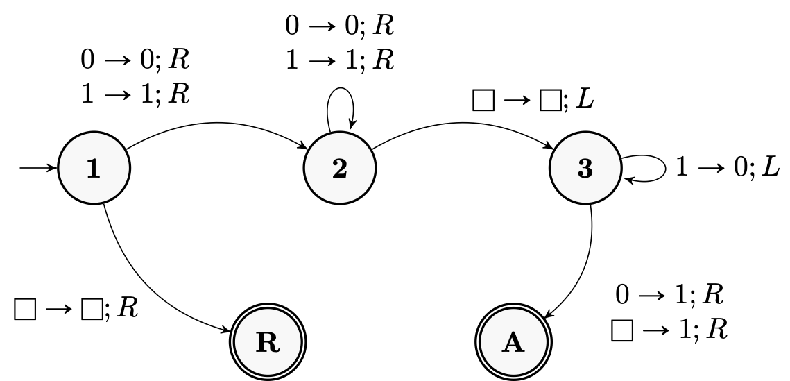
The edges in the diagram describe all the actions that a Turing machine can do in a computational step. For example, the self-loop in the top right corner of the diagram above specifies that if the machine is currently in state \(\mathbf{3}\) and the tape head is over a square with the symbol \(1\), it writes a \(0\) on that square (overwriting the previous \(1\)), moves the tape head Left one square, and stays in state \(\mathbf{3}\).

We can also provide a formal definition of Turing machines in the following way.

Definition. A deterministic one-tape Turing machine is an abstract machine described by the triple

\[M = (m,k,\delta)\]

with $m,k \ge 1$ where

• \(\mathbf{Q} = \{\mathbf{1}, \mathbf{2}, \ldots, \mathbf{m}\}\) is the set of internal states,
• \(\Gamma = \{\square,0,1,2,\ldots,k\}\) is the tape alphabet, and
• \(\delta \colon \mathbf{Q} \times \Gamma \to (\mathbf{Q} \cup \{\mathbf{A}, \mathbf{R}\}) \times \Gamma \times \{L, R\}\) is the transition function.

The state \(\mathbf{1}\) denotes the initial state of the Turing machine \(M\). (We will use bold symbols to denote the states of the machine, to prevent any confusion with the symbols used on the tape.)

In order to simulate a Turing machine, we need to keep track of its internal state, the current string on the tape, and the position of the tape head on the tape. We call this information the configuration of a Turing machine. It can be represented conveniently in the following way.

Definition. The configuration of a Turing machine is a string \(w \mathbf{q} y\) where

• \(\mathbf{q} \in \mathbf{Q} \cup \{ \mathbf{A}, \mathbf{R} \}\) represents the current state of the machine,
• \(wy \in \Gamma^*\) is the current string on the tape, and
• the position of the tape head is on the first symbol of \(y\).

Two configurations are equivalent when they are identical up to blank symbols at the beginning of \(w\) or at the end of \(y\). In other words, they satisfy

When \(\mathbf{q} = \mathbf{A}\), the string \(w \mathbf{q} y\) represents an accepting configuration. When \(\mathbf{q} = \mathbf{R}\), it represents a rejecting configuration. A configuration is a halting configuration if it is either accepting or rejecting.

A step of computation of a Turing machine typically changes its configuration. We can simulate a Turing machine by listing the configurations obtained after each computation step. For example, when running the Turing machine in the diagram above on the input \(1011\), the following sequence of configurations are obtained:

Note that the additional spacing in the representation of the configurations is not required by the definition, but it does make it easier to follow the simulation of the Turing machine. Note also that for clarity the blank squares on the tape are written explicitly only when they are required (as is the case in the step above where the tape head is positioned over a blank square).

A list of the configurations obtained during the execution of a Turing machine is called a tableau. We can also formally define which configurations follow each other in the execution of a Turing machine in the following way.

Definition. For any strings \(w,y \in \Gamma^*\), symbols \(a,b,c \in \Gamma\), and states \(\mathbf{q} \in \mathbf{Q}\) and \(\mathbf{r} \in \mathbf{Q} \cup \{ \mathbf{A}, \mathbf{R} \}\), the configuration \(wa\mathbf{q}by\) of the Turing machine \(M\) yields the configuration \(w \mathbf{r} acy\), denoted

\[wa \mathbf{q} by \vdash w \mathbf{r} acy\]

when \(\delta(\mathbf{q},b) = (\mathbf{r},c,L)\). Similarly,

\[wa \mathbf{q} by \vdash wac \mathbf{r} y\]

when \(\delta(\mathbf{q},b) = (\mathbf{r},c,R)\).

By simulating multiple steps of computation, a Turing machine can reach some other configurations. Specifically, we say that the configuration \(w \mathbf{q} y\) derives the configuration \(w' \mathbf{q'} y'\) in the Turing machine \(M\), denoted

when there exists a finite sequence of configurations \(w_1 \mathbf{q}_1 y_1, \ldots, w_k \mathbf{q}_k y_k\) such that

The Turing machine \(M\) accepts an input \(x \in \{0,1\}^*\) if the initial configuration \(\mathbf{1}x\) derives an accepting configuration. It rejects \(x\) if \(\mathbf{1}x\) derives a rejecting configuration. And it halts on \(x\) if and only if it either accepts or rejects \(x\).

With these definitions in place, we can now formally define what it means for a Turing machine to “compute” a language.

Definition. The Turing machine \(M\) decides the language \(L \subseteq \{0,1\}^*\) if it accepts every \(x \in L\) and rejects every \(x \notin L\).

A language is decidable if and only if there is a Turing machine that decides it. (The set of all decidable languages is also known as the set of recursive languages.)

Note that the definition is equivalent to requiring the deciding Turing machine to always halt on all inputs and to accept if and only if the input is in the language. If we relax the requirement that the Turing machine must halt on all inputs but keep the requirement that the set of inputs accepted by the machine \(M\) is exactly the set of strings in a language \(L\), we obtain a weaker notion of computation that we denote by saying that \(M\) recognizes the language \(L\).

Universal Turing Machine

Turing machines can decide many simple languages, and to become familiar with them it is a useful exercise to design Turing machines for your favourite one. (E.g., can you design a Turing machine to decide the language of all palindromes? Of all strings that contain more \(1\)s than \(0\)s? Of the strings that represent the binary encodings of powers of \(3\)?)

But Turing machines can also accomplish surprisingly complex tasks. Perhaps the most far-reaching such result, first established by Alan Turing himself, is that there is a Universal Turing Machine that can simulate all other Turing machines. To properly introduce the universal Turing machine, we start with a basic observation.

Proposition 1. There is an encoding that maps each Turing machine \(M\) to a binary string \(\left< M \right> \in \{0,1\}^*\).

Proof. The proposition is an immediate consequence of the fact that Turing machines have a finite description.

Or we can describe an explicit encoding in the following way. Consider the machine \(M = (m,k,\delta)\). The positive integers \(m\) and \(k\) can be encoded by taking their binary representation. And the transition function \(\delta\) can be represented as a table of $m \cdot (k+2)$ entries (one for each internal state-tape symbol pair). Each of these entries can be encoded as a binary string. We can combine all these elements into a single binary representation to obtain the final encoding of \(M\).

We say that a Turing machine \(S\) simulates machine \(M\) on input \(x \in \{0,1\}^*\) when \(S\) accepts if and only if \(M\) accepts \(x\), \(S\) rejects if and only if \(M\) rejects \(x\), and in both cases \(S\) ends with the same content on the tape as \(M\) does.

We can now show that there exists a single Turing machine that can simulate all the other ones in the following precise sense.

Theorem 2. There is a Universal Turing Machine \(U\) such that for every Turing machine \(M\) and every input \(x \in \{0,1\}^n\), when the input to \(U\) is the string \(\left< M \right> x\) then \(U\) simulates the execution of \(M\) on input \(x\).

Proof. We give a high-level description of \(U\). A quick warning: it is not immediately clear how all the steps below can be implemented using Turing machines. For a great exercise, see if you can fill out the details for the implementation of some of these steps.

As a first step, the machine \(U\) turns the input \(x\) into the initial configuration of \(M\) by adding a special symbol \(\mathbf{1}\) at the beginning of \(x\) to turn it into the string \(\mathbf{1}x\). Then it proceeds to simulate the execution of \(M\) step by step. Each computational step is simulated by following a 3-stage process.

1. Read the current state \(\mathbf{q}\) and the symbol \(a\) at the tape head in \(M\)’s current configuration.
2. Go back to the encoding \(\left< M \right>\) of \(M\) to read the entry \(\delta(\mathbf{q},a)\) of its transition table.
3. Update the configuration appropriately by overwriting the symbol \(a\) at the tape head position, moving the tape head left or right, and updating the current state of the machine.

The machine \(U\) continues simulating \(M\) until the latter halts. At this point, \(U\) erases the encoding \(\left<M\right>\) of \(M\) from the tape and the current state in the configuration string. This leaves the tape in the same state as \(M\)’s tape when it halts, and \(U\) halts by accepting or rejecting to mimic the halting state of \(M\).

The existence of a Universal Turing Machine is a remarkable result, and one that will return many times throughout this course. As a very first application, we can use it to examine a strong claim: that Turing machines are as powerful as any types of computational machines.

Church-Turing Thesis

Let us now examine the claim that Turing machines are general enough to capture the notion of what is computable by all other reasonable models of computation. The claim itself is known as the Church-Turing Thesis.

Church-Turing Thesis. Any decision problem that can be solved by any computer that respects the laws of physics corresponds to a language that can be decided by a Turing machine.

We can’t prove the Church-Turing thesis, but we can certainly test it out with any reasonable model of computation that we can imagine. Here’s a simple such test.

A counter machine is a machine that has \(k\) registers (for some finite \(k \ge 1\)) that each hold an integer. Importantly, the integers in these counters (unlike the ones in the computers we usually work with) are unbounded. The input to the counter machine is the binary representation of the number stored in the first register when it starts; all other registers initially hold the value \(0\). A counter machine program is a finite list of operations from the following list:

• \(\texttt{CLR}(r)\) clears register \(r\) by setting it to \(0\).
• \(\texttt{INC}(r)\) increments the integer in register \(r\).
• \(\texttt{DEC}(r)\) decrements register \(r\).
• \(\texttt{CPY}(r,s)\) copies register \(r\) into register \(s\).
• \(\texttt{JMP}(a)\) jumps to the \(a\)th instruction in the program.
• \(\texttt{JZ}(a,r)\) jumps to the \(a\)th instruction if register \(r\) equals zero.
• \(\texttt{HALT}\) halts the execution of the program.

A counter machine program computes the language \(L \subseteq \{0,1\}^*\) when it halts on all inputs and has a non-zero value in register \(1\) upon halting if and only if its input was in \(L\).

As you can verify directly, counter machines can compute many non-trivial languages. (In fact, though we will not prove it, they can compute all decidable languages.) But using the same ideas as we used in the design of the Universal Turing Machine, we can show that all of the languages that can be computed by counter machines are indeed also computable by Turing machines.

Proposition 3. Every language \(L \subseteq \{0,1\}^*\) that can be computed using counter machines can also be decided by a Turing machine.

Proof. We use the same idea as in the proof of the existence of a Universal Turing Machine: if you give me the description of a counter machine program, I can simulate the program with a Turing machine. Again, we give only a high-level description of the simulation.

Fix a counter machine program \(P\). We can initialize our simulation of \(P\) on some input \(x\) by writing the binary representation of \(k\) integers on tape: the input \(x\) itself is in the first stored register, and the other \(k-1\) ones are initialized to \(0\). We also add another counter on the tape to keep track of the current step of the program we are executing. We then simulate the execution of \(P\) step by step.

Each \(\texttt{CLR}\), \(\texttt{INC}\), \(\texttt{DEC}\), and \(\texttt{CPY}\) operation can be implemented by modifying the appropriate register value on the tape directly. The \(\texttt{JMP}\) operation is simulated by changing the value of the counter that keeps track of our current step in the execution of the program. And the \(\texttt{JZ}\) operation is very similar, except that we add an extra check on the appropriate register and skip the jump if that register does not hold a zero.

Finally, when the counter machine program \(\texttt{HALT}\)s, we terminate the simulation, check the value in the first register stored on tape. We accept if that value is non-zero and reject otherwise.

The proof of the proposition gives the template for confirming the Church-Turing thesis on any other model of computation that you could define: to prove that Turing machines capture that model of computation, it suffices to show how to simulate the programs on these computers using a Turing machine.

Incidentally, you can use the same approach to show that any other model of computation is as powerful as Turing machines (and so, by the Church-Turing thesis, as powerful as any other reasonable model of computation!): simply show how Turing machines can be simulated in your model. Every model of computation for which this task can be completed is called Turing-complete.

Eric Blais ©2024 — Last edited on Jan. 10, 2024