2 Propositional Logic
\(\newcommand{\la}{\lambda} \newcommand{\Ga}{\Gamma} \newcommand{\ra}{\rightarrow} \newcommand{\Ra}{\Rightarrow} \newcommand{\La}{\Leftarrow} \newcommand{\tl}{\triangleleft} \newcommand{\ir}[3]{\displaystyle\frac{#2}{#3}~{\textstyle #1}}\)
Statistically, we is OK, ’cause our laughing man is one of the crowd.
(Wake Up, Essential Logic, 1979)
It is traditional to study logic in stages, and the first stage, propositional logic, is relatively straightforward. Most of the difficulty we will encounter will be in developing the discipline and notation to be precise.
The idea of being more precise about the rules of argument goes back to the Greek philosopher Aristotle (4th century BCE), with further development by Peter Abelard in the Middle Ages and by Gottfried Leibniz in the 17th century. The historical figures who contributed to the development of logic are often fascinating objects of study in their own right. Aristotle was a huge influence on the development of Western thought, in both the sciences and the humanities. One interesting tidbit: he was the tutor of Alexander the Great. Abelard’s tragic romance with Héloïse d’Argenteuil has made their shared crypt in Paris a popular tourist destination, and Leibniz you probably know as the co-inventor of calculus.
Tempting though it is to expand on these stories, I will let you look them up on your own. I have some suggestions of good references in the Resources chapter.
The discussion of divisibility in the introduction suggests that we need three things: a language with which to make precise logical statements, a precise definition of what constitutes a valid proof of such a statement, and a program that will check a given proof for validity. Our goal is to design the second (definition of proof) so that the third (the program) is short and simple to write.
Let me paraphrase the definition of divisibility and the theorem I quoted, with some changes that bring us closer to the level of precision we’re after.
Divisibility: \(m \mid n\) means there exists an integer \(k\) so that \(n = (k~*~m)\). Here I have made the multiplication explicit, and added parentheses which we will use in the theorem to group operations.
Divisibility of Integer Combinations (DIC): For integers \(a,b,c\), if \(a \mid b\) and \(a\mid c\), then for integers \(x,y\), \(a \mid ((b*x)+(c*y))\).
These are quite readable, but in formalization, we typically define even more concise and precise notation. For example, we can represent the set of integers by the symbol \(\mathbb{Z}\), and replace the statement "\(a\) is an integer" with the set-theoretic notation \(a\in\mathbb{Z}\) (read as "\(a\) is an element of \(\mathbb{Z}\)"). The definition of divisibility becomes \(\exists k \in \mathbb{Z}, ~n=(k*m)\), using the symbol \(\exists\) to replace "there exists". This is a logical statement or formula expressing a relationship between \(n\) and \(m\). The statement of DIC becomes:
"For all \(a,b,c\in\mathbb{Z}\), if \(a \mid b\) and \(a\mid c\), then for all \(x,y\in\mathbb{Z}\), \(a \mid ((b*x)+(c*y))\)."
Continuing to replace English words, we can use the symbol \(\forall\) for "for all", the symbol \(\land\) for "and", and the symbol \(\ra\) for implication ("if/then"):
\(\forall a,b,c\in\mathbb{Z}, ((a \mid b) \land (a\mid c) \ra (\forall x,y\in\mathbb{Z}, a \mid (bx+cy)))\).
Some of the things in this logical formula, like \(\ra\) and \(\land\), we will discuss in this chapter. Others, like \(\forall\), \(\exists\), numbers, and arithmetic operations, we will put off to the next chapter.
But before we defer arithmetic operations, we can use them as a simple example to illustrate how we’re going to be precise about language and proof. Let’s consider arithmetic expressions made up of numbers, addition, and multiplication. A common way to describe such things in computer science is to use a grammar. For example, this is how the Racket teaching languages are described in the documentation.
The grammar for arithmetic expressions looks like this.
| E | = | n | ||
| | | (E + E) | |||
| | | (E * E) |
There are three grammar rules. We could write each one beginning E =, but the notation instead uses a vertical bar (|) for subsequent rules. The symbol = does not mean equality here; it should be read as "can be", indicating a possible refinement of E.
The first grammar rule says that any integer by itself is an arithmetic expression (using the extreme shorthand that n is often used as a generic name for an integer). The second says that the parenthesized sum of two arithmetic expressions is an arithmetic expression, and the third does the same for the product of two arithmetic expressions.
Any given arithmetic expression, such as \(((1+2)*(3+4))\), can be justified by the grammar rules. "\(((1+2)*(3+4))\) is an arithmetic expression because \((1+2)\) and \((3+4)\) are arithmetic expressions," followed by justifications for those subexpressions. We can build these justifications out of the following three translations of the rules:
If \(n\) is an integer, then \(n\) is an arithmetic expression.
If \(E_1\) and \(E_2\) are arithmetic expressions, then \((E_1+E_2)\) is an arithmetic expression.
If \(E_1\) and \(E_2\) are arithmetic expressions, then \((E_1*E_2)\) is an arithmetic expression.
These justifications are essentially proofs that a given expression is an arithmetic expression. Although we will be using grammars to describe our logical languages from now on, we can use this example to introduce the notation we will be using to describe proof rules. Each of these rules has a conclusion that is drawn from some premises. Such a rule is called an inference rule. We can write each rule using a horizontal line with the premises above and conclusion below. For further brevity, we can use set notation, defining \(\mathcal{E}\) as the set of arithmetic expressions.
\[\ir{}{n \in \mathbb{Z}}{n \in \mathcal{E}} ~~ \ir{}{E_1 \in \mathcal{E} ~~~ E_2 \in \mathcal{E}}{(E_1 + E_2) \in \mathcal{E}} ~~ \ir{}{E_1 \in \mathcal{E} ~~~ E_2 \in \mathcal{E}}{(E_1 * E_2) \in \mathcal{E}}\]
There is a subtlety here that is worth highlighting. In the grammar, I could use E twice in one rule, and each use is independent (those expressions could be the same or different). That’s part of the way we interpret grammar rules. But, more generally, with inference rules, we might want to refer to the same thing twice. So two uses of \(E\) in an inference rule would refer to the same thing. Because I want to match the "could be the same or different" behaviour of the grammar, I have to use \(E_1\) and \(E_2\) in my inference rules.
These rules can be applied to specific expressions. Here is a use of a rule concluding that \(((1+2)*(3+4))\) is an arithmetic expression.
\[\ir{}{(1+2) \in \mathcal{E} ~~~ (3+4) \in \mathcal{E}}{((1+2) * (3+4)) \in \mathcal{E}}\]
This is not a complete proof, because we don’t have justification for the premises. We can justify, say, \((1+2) \in \mathcal{E}\) by another use of a rule with this as the conclusion. But since it is also used as a premise above, we can save space by putting the two uses together. Continuing the process, we arrive at the complete justification below.
\[\ir{} {\ir{}{\ir{}{1 \in \mathbb{Z}}{1 \in \mathcal{E}} ~~ \ir{}{2 \in \mathbb{Z}}{2 \in \mathcal{E}}}{(1+2) \in \mathcal{E}} ~~~ \ir{}{\ir{}{3 \in \mathbb{Z}}{3 \in \mathcal{E}} ~~ \ir{}{4 \in \mathbb{Z}}{4 \in \mathcal{E}}}{(3+4) \in \mathcal{E}}} {((1+2) * (3+4)) \in \mathcal{E}}\]
This is a tree, because each use of a rule has only one conclusion but can have several premises. Proof trees like this are traditionally drawn with the conclusion at the bottom. Formally, a proof tree is an application of an inference rule together with proof trees for all the premises of that rule. This is a recursive definition of "proof tree".
More generally, in computer science, trees are usually drawn with the root at the top instead of the bottom. If we flip this tree over and trim away redundant information, it might look like this:
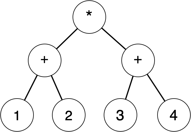
This is often called a "parse tree", and the creation of one from a string of characters such as "((1+2)*(3+4))" is called "parsing". In general, this is a complex subject about which many books have been written, but because of our liberal use of parentheses, it is not difficult to construct the parse tree from the string in this case. That is also the reason behind the use of parentheses in Racket.
The tree form is convenient for manipulating such expressions, for example in evaluating them to a single number. There are many choices for representing a tree, but in Racket it is convenient to use nested lists. We can represent the tree above as (list '* (list '+ 1 2) (list '+ 3 4)) or, using quote notation, as '(* (+ 1 2) (+ 3 4)). Notice that this looks a lot like Racket code. This is one of the reasons that Racket is well-suited for use in this stroll. We don’t have to work hard to parse a string of characters into a data structure suitable for manipulating the expression; we can just put a single quote at the front of it.
We won’t be working with arithmetic expressions in what follows, but the same techniques work very nicely for logical formulas and proof trees. We will be representing both of these using nested lists in Racket.
A set of related inference rules, such as the ones for membership in \(\mathcal{E}\) given above, give us a recursive definition of a set of trees, namely the set of trees that can be constructed by applications of the rules. It also gives us a recursive definition of the set of things that can be proved using the rules, namely the conclusions at the roots of those trees. We can define functions on these sets by structural recursion, and prove things about these sets by structural induction. We will be doing these things shortly.
2.1 Formulas
The formulas that we will study in this chapter resemble arithmetic expressions. In place of \(+\) and \(*\), we have logical connectives. We’ve already seen \(\land\) (and/conjunction), and \(\ra\) (if-then/implication). The other two are \(\lor\) (or/disjunction), and \(\lnot\) (not/negation).
In place of the integers we used in arithmetic expressions, we have propositional variables \(A,B,C\ldots\). The variables represent statements or atomic propositions. These need not be mathematical propositions; they might be statements such as "Waterloo is in Canada". These statements have been abstracted away, just as numbers are abstracted away by the use of algebraic variables. The connectives are used to form compound statements, such as \(A \land B\) and \((\lnot B) \ra (A \lor C)\). This is the language of propositional logic.
Other connectives are sometimes used. You may be familiar with "if and only if", or "iff" for short; \(\leftrightarrow\) is used to represent this. However, we can express this using the connectives above: \(A \leftrightarrow B\) is the same as \((A \ra B) \land (B \ra A)\).
Here is the grammar of propositional formulas. We will be adjusting this grammar as we go, but this will do as a start.
| T | = | X | ||
| | | (T ∧ T) | |||
| | | (T ∨ T) | |||
| | | (¬ T) | |||
| | | (T → T) |
In the first rule, we are using X to stand in for any possible variable, just as we earlier used n to stand in for any possible integer. We call X a metavariable, since it is a variable ranging over other variables. To limit confusion, I will try to use capital letters late in the alphabet (such as \(X\)) as metavariables, and those early in the alphabet (such as \(A,B,C\ldots\) which I used above) as actual variables in examples.
In practice, it’s useful to have an unbounded number of variables, so we might use natural number subscripts, such as \(A_i\). This facilitates using variables to describe parts of finite but unbounded structures. For example, we could generalize a checkerboard from \(8\times 8\) to \(n \times n\), and then use \(B_{i,j}\) to represent the statement "there is a checker on square \((i,j)\)". While you may encounter such notation outside this stroll, we will not need to use it here.
For readability, we usually display a formula as a linear sequence of symbols, just as with arithmetic expressions. But it’s important to keep in mind that a formula is really a tree, and that is the representation we will use internally in our Racket programs.
Is an informal proof, such as the one I quoted in the introduction, really a tree? We tend to write such proofs out in a linear fashion also. Some formalizations of proof that you may see in other references do the same thing, perhaps numbering each application of a rule, so that application #13 makes use of the conclusions of applications #4 and #8. This is economical with space, but we could unwind such a proof so that every time we need to use conclusion #8, we repeat the complete proof of #8 entirely from scratch. If we do this systematically, we would get a tree. The point is that other formalizations may be more concise, but they are not more powerful.
The consistent use of parentheses in formulas can be awkward for humans. For arithmetic expressions, there are conventions to reduce parentheses, such as performing multiplication before addition. These conventions allow us to write \(((5*6)+(7*8))\) as \(5*6+7*8\). There are similar conventions to reduce the number of parentheses in displayed formulas. We will call the resulting simplified syntax human-readable, and I’ll be using it on these web pages. (Later, for working with Proust, we will restore some (but not all) of the parentheses to facilitate the use of quote notation and simplify the code, resulting in a third variation of syntax.)
We can remove the outermost parentheses of any formula. We can consider \(\ra\) to be right-associative, so we can write \(A\ra B \ra C\) instead of \(A\ra (B \ra C)\). We can assign precedence among operators, just as we do with addition and multiplication in algebra, and remove parentheses made redundant by operators of higher precedence being used first to form expressions. For formulas, \(\lnot\) has the highest precedence and \(\ra\) the lowest, with \(\land\) and \(\lor\) with the same (middle) precedence (and left-associativity).
When making precise a mathematical statement such as DIC above, we have at least an informal notion of what it means for such a statement to hold. But since we have abstracted away so much, it’s no longer clear what it means for a propositional formula to hold. We don’t know what its propositional variables are referring to. In the next section I will describe the most common way of providing this meaning. But it will play a reduced role in our journey. I am bringing it up early because it may already be in your head, and I hope to convince you to put it to one side for a while.
2.2 The Boolean interpretation
In your programming experience, you will have encountered conditional expressions. These start with tests, such as a test of equality between two integer variables. These tests can take on one of two values, some variation on "true" and "false". The tests can be combined by some variation of the logical connectives we’ve discussed, typically "and", "or", and "not". The evaluation of some specified code can be made conditional on the result of the combination being "true".
In Racket, the two values are #t and #f, and the connectives are functions (or macros) and, or, not. In the C programming language, the two values are 1 and 0, and the connectives are operators &&, ||, and !. Many presentations of logic use T and F to represent the two values. We will use 1 and 0 here, to avoid confusion with variables in formulas and metavariables in inference rules. Using 1 and 0 is also done in circuit design and discussions of computer design and architecture.
1 and 0 were also used by the Scottish mathematician George Boole in the 1850’s when he defined the mathematical concepts that led to his name being associated with these values. The two values (regardless of their representation) are called Boolean values. Boole’s book The Laws of Thought (1854) introduced what is now called Boolean algebra. It was edited by his wife Mary Everest, whom he tutored privately in mathematics. George died relatively young; Mary went on to write several books on mathematics education and to be a private tutor herself (she could not be a professor like George; there were no women professors in the UK in the 19th century).
The connectives in the programming languages are functions that consume one or two Boolean values and produce one Boolean value. Their computational meaning can be given by a table of values for all choices of arguments. For Boolean operators, this table is called a truth table. We will overload symbols, so that \(\land\) will refer both to the logical symbol in a formula and to the Boolean binary operator. Here are the truth tables for the Boolean functions. Note the order of rows, with 1 coming before 0 and the rightmost variable varying fastest; this is a standard convention for truth tables.
\(x\) |
| \(y\) |
|
|
| \(x\land y\) |
1 |
| 1 |
|
|
| 1 |
1 |
| 0 |
|
|
| 0 |
0 |
| 1 |
|
|
| 0 |
0 |
| 0 |
|
|
| 0 |
\(x\) |
| \(y\) |
|
|
| \(x\lor y\) |
1 |
| 1 |
|
|
| 1 |
1 |
| 0 |
|
|
| 1 |
0 |
| 1 |
|
|
| 1 |
0 |
| 0 |
|
|
| 0 |
\(x\) |
| \(y\) |
|
|
| \(x\ra y\) |
1 |
| 1 |
|
|
| 1 |
1 |
| 0 |
|
|
| 0 |
0 |
| 1 |
|
|
| 1 |
0 |
| 0 |
|
|
| 1 |
\(x\) |
|
|
| \(\lnot x\) |
1 |
|
|
| 0 |
0 |
|
|
| 1 |
Intuitively, the AND of two values is 1 exactly when they are both 1; the OR of two values is 1 exactly when at least one of them is 1; and the NOT of a value is 1 exactly when the value is 0. Continuing the intuitive discussion, we can assign a Boolean value to a propositional formula by assigning a Boolean value to each of its propositional variables and interpreting its connectives as the corresponding Boolean function. We will say that a propositional formula is true exactly when any possible assignment results in the formula evaluating to true.
It’s important to keep in mind that a logical formula is just a tree of symbols. The interpretation is up to us. This interpretation is useful, and you already have some sense of it because of your programming experience. But it is not the only possible interpretation. The grammatical definition of a formula gives us syntax, and the Boolean interpretation gives us semantics (meaning), but other semantic definitions are possible, and we will see some of them. But first, let’s formalize the Boolean interpretation.
For the assignment of Boolean values to variables, we use a valuation \(v\), which is a map or function from propositional variables to \(\{0,1\}\). For applying the connectives, we use a recursive definition for \(\langle T \rangle_v\), which is the truth value assigned to formula \(T\) by valuation \(v\).
\begin{align*}\langle X \rangle_v &= v(X), ~X\mbox{ a variable}\\ \langle T \land V \rangle_v &= \langle T \rangle_v \land \langle V \rangle_v \\ \langle T \lor V \rangle_v &= \langle T \rangle_v \lor \langle V \rangle_v \\ \langle T \ra V \rangle_v &= \langle T \rangle_v \ra \langle V \rangle_v \\ \langle \lnot T \rangle_v &= \lnot \langle T \rangle_v\end{align*}
We say a formula \(T\) is true if and only if for all valuations \(v\), \(\langle T \rangle_v = 1\). As a simple example of using the Boolean interpretation, \(A \ra \lnot \lnot A\) is true. There are only two valuations to consider, \(v(A) = 1\) and \(v'(A) = 0\), and working through the definitions confirms \(\langle A \ra \lnot \lnot A \rangle_v = 1\) and \(\langle A \ra \lnot \lnot A \rangle_{v'} = 1\).
Even this small calculation is tedious, and if there were more variables, the calculation would become large. We have computers to automate tasks like this, but since the number of valuations is exponential in the number of variables used, we are going to run into efficiency issues. I mentioned in the Introduction that proof exists as an alternative to exhaustive case analysis. What we need here is an idea of proof (that a formula is true) that does not involve checking all valuations. We will spend most of the rest of this chapter developing that idea, but I want to talk about it abstractly first.
In your experience with mathematical proof, you may have been encouraged to blur the line between truth and proof. You might have been shown techniques that in effect used truth value (in the Boolean interpretation) as a guide to local manipulation of logical statements in proofs. For example, you might have seen a case where a statement of the form "not-B implies not-A" is replaced by "A implies B".
This is permitted, as it turns out, because for classical logic, this notion of truth coincides with the notion of proof, in a way that is not true for intuitionistic logic. On hearing this, you may well ask, "Then why are we using intuitionistic logic?". The main reason is that it leads to a computational interpretation that has proven important in proof assistant software, but it was considered a preferable alternative by many mathematicians long before proof assistants (or even computers) came along. I won’t attempt to justify the choice completely right now; that will happen over the course of our stroll. But let’s tease apart this notion of truth and proof coinciding, just a bit.
We haven’t yet been at all precise about proof, but there are two important ways that proof and truth can be related. The statement "If a formula has a proof, then it is true in our chosen interpretation" is called soundness. Soundness is important, because without it, there is really no point in doing proof. Intuitively, soundness confirms that our proof rules are sensible, and that we can’t prove something that isn’t true. The contrapositive of the above statement of soundness, "If a formula is not true, then it has no proof", can be useful in saving us the trouble of searching for a non-existent proof, if we have a simple demonstration that a formula is not true (e.g. a counterexample). Proofs of soundness can be fairly straightforward.
The statement "If a formula is true, then it has a proof" is called completeness. This is mathematically interesting, but practically less important. Just because that proof exists doesn’t mean it is short, illustrative, or can be easily constructed. With respect to the Boolean interpretation, classical logic is sound and complete; however, intuitionistic logic is sound but not complete. Proofs of completeness (when possible) tend to be more complicated than proofs of soundness. Completeness isn’t possible for any logic strong enough to say anything interesting about mathematics or computer science (we will discuss this further in the next chapter), so we eventually have to do without it anyway.
As I said above, the Boolean interpretation of truth is not the only one possible. Without going into too much detail, I can give a quick example of another interpretation. Fix a set \(X\), and let a valuation be a map from variables to subsets of \(X\). We can then define the notion of a truth value for formulas by interpreting \(\lor\) as \(\cup\) (set union), \(\land\) as \(\cap\) (set intersection), and \(\lnot\) as complement with respect to \(X\). The interpretation of \(T\ra W\) is a little more complicated; it is the union of the interpretation of \(W\) with the complement of the interpretation of \(T\). We say a formula \(T\) is true if for all valuations \(v\), \(\langle T \rangle_v=X\).
This is a generalization of the Boolean valuation, since if \(X\) has only a single element, the resulting interpretation is the Boolean valuation. But \(X\) can have more than one element, so it is a generalization. It is possible to show that for classical logic, this new notion of truth also coincides with proof (that is, we can prove soundness and completeness). But for intuitionistic logic, once again, we can prove soundness but not completeness. However, with a little tweak to this new interpretation, we can get a notion of truth that coincides with proof for intuitionistic logic, that is, we can prove both soundness and completeness. I won’t discuss this tweak further at the moment, but later on I will describe yet another notion of truth suitable for intuitionistic logic, and we will work with it to demonstrate the unprovability of certain formulas.
The point of this discussion is to persuade you to put away the Boolean interpretation and focus on proof. Please keep the notion of truth out of your head until I explicitly bring it up. This may not be easy. It might feel a little like keeping the idea of mutation out of your head while learning Racket from HtDP, TYR, or FICS. But just as there was benefit in doing that, there will be benefit in doing this. Nicolaas de Bruijn (about whom we will hear more later) once wrote, "Boolean logic is metatheory of classical reasoning. NOT reasoning itself." We’ll come back to this point.
Let’s talk about proof in detail now.
2.3 Proof for the implicational fragment
We’ll start by restricting the language of formulas to consider formulas built from only propositional variables and implication. Later we’ll add in the other connectives one at a time.
| T | = | X | ||
| | | (T → T) |
How do we informally prove a statement of the form \(T \ra W\)? As discussed in the Introduction, the direct method is to assume \(T\) and use the assumption to prove \(W\). In the course of proving \(W\), we have to remember that we assumed \(T\). Since \(W\) may itself be an implication, the assumptions are going to accumulate during the proof process. At any point, we may have to remember a set of assumptions, not just one.
This suggests working out inference rules for when a provability relation holds between a set of assumptions and a formula. The relation will mean "this set of assumptions can be used to prove this formula". It will hold for some sets of assumptions and associated formulas, and not for others.
We’ll introduce new notation with a new symbol for this relation. We write \(\Gamma\vdash T\) to mean "From the assumptions in \(\Gamma\), we can prove \(T\)", or, more briefly, "\(\Gamma\) proves \(T\)." A statement of this form is called a sequent, and the set \(\Gamma\) is often called a context. The symbol \(\vdash\), often called "turnstile", comes from the writings of Gottlob Frege, who was the first to address predicate logic in symbolic terms in 1879. The idea of sequents is due to Gerhard Gentzen, who in 1934 introduced the system of natural deduction that we will study. I’ll discuss the historical context of Frege and Gentzen later in this stroll, after we’ve learned a little bit more about their ideas.
From the discussion above, there are times when we might need to add a new assumption to a context. We could use set notation and write \(\Gamma \cup \{T\}\). But it is standard to use a different notation for the same idea, and to write \(\Gamma,T\) for this. Also, we will write \(\emptyset\vdash T\) as \(\vdash T\).
We can write down any sequent we want, but only certain ones will be valid, because they will have proof trees using inference rules that we will work out. Here is the inference rule resulting from the above discussion, the first one in our accumulating set of inference rules for natural deduction. The label \(\ra_I\) is short for "implication introduction".
\[\ir{(\ra_I)}{\Gamma,T\vdash W}{\Gamma\vdash T\ra W}\]
How do we use or "eliminate" an implication? If we know \(T\ra W\) and we know \(T\), we can conclude \(W\). This rule is called "modus ponens", which is Latin, so you know it’s really old. (It comes from the Peripatetic School of Aristotle in the 3rd century BCE.) Here’s what it looks like in modern notation. The label \(\ra_E\) is short for "implication elimination".
\[\ir{(\ra_E)}{\Gamma\vdash T\ra W ~~~ \Gamma\vdash T}{\Gamma\vdash W}\]
We need a way of using assumptions in contexts. A context containing the assumption \(T\) proves \(T\).
\[\ir{(\mbox{Ass})}{T \in \Gamma}{\Gamma\vdash T}\]
Here’s a slick way of writing this rule that makes it clear it’s an axiom; that is, it has no premises, or its premises do not need proving by the application of another inference rule. Axioms form the leaves of a proof tree.
\[\ir{(\mbox{Ass})}{}{\Gamma,T\vdash T}\]
These three rules of natural deduction are enough to prove some formulas that only involve implication. Here’s an example of a proof tree, for the formula \(A \ra (B \ra A)\).
\[\ir{(\ra_I)} {\ir {(\ra_I)} {\ir {(\mbox{Ass})} {} {A,B \vdash A}} {A \vdash B \ra A}} {\vdash A \ra (B \ra A)}\]
This is a tree, but it doesn’t branch, because the \(\ra_I\) inference rule has only one premise. It’s best to read these trees bottom to top. At the bottom is the final conclusion, under a horizontal line, and above it are the subgoals we need in order to reach that conclusion with the final application of a rule. Above each of those are further subgoals, and so on.
The tree below, for the formula \(A \ra ((A \ra B) \ra B)\), has a branch in it, because the \(\ra_E\) inference rule has two premises.
\[\ir{(\ra_I)} {\ir {(\ra_I)} {\ir {(\ra_E)} {\ir {(\mbox{Ass})} {} {A,A\ra B\vdash A\ra B} ~~~\ir {(\mbox{Ass})} {} {A,A\ra B\vdash A}} {A,A\ra B\vdash B}} {A \vdash (A \ra B) \ra B}} {\vdash A \ra ((A \ra B) \ra B)}\]
Even though this is a small example, you can see that proof trees rapidly become awkward to work with. We will introduce a better representation below, but you should not forget that better representations represent these trees. I will stop drawing proof trees once we have that better representation, but you should be able to reconstruct the trees.
So far we have not deviated from a conventional treatment, though another reference might have different names for the rules and a different representation for the proof tree. Since we know how to represent trees in Racket, we could easily describe a Racket representation for proof trees, and write a proof checker which checks the validity of a supplied proof tree.
Introducing the idea of proofs as programs opens up a small but significant gap between our approach and others, a gap that we will continue to widen. Before we do this, let me briefly mention some other systems of proof.
Hilbert-style systems for propositional logic (named after David Hilbert, a major figure in the formalization of mathematics in the late 19th and early 20th Centuries) have modus ponens as the only inference rule with premises; everything else is an axiom. This simplifies some metamathematics, such as proofs of soundness and completeness, by cutting down on cases. But proofs in such a system do not look much like informal proofs in mathematics.
At the same time that Gentzen introduced natural deduction (so named because it more closely resembles informal proof), he also introduced another system called the sequent calculus, which has even more rules, but is more symmetrical, and consequently also good for metamathematics. Both of these alternatives (Hilbert-style, and sequent calculus) are worth studying, but we will not consider them here.
2.4 Proofs as programs
The Boolean interpretation centres the notion of truth. Each connective is interpreted in terms of the truth value of a formula that is built using that connective at the root of the tree. If we downplay the notion of truth, we must instead reason intuitively about what proofs of formulas should look like. That is: we interpret each of the logical connectives in terms of what a proof of a formula using that connective should look like.
This is the basis of the BHK interpretation, named after the three mathematicians who formulated it. Dutch mathematician L.E.J. Brouwer, in the early 20th century, reacted to Hilbert’s formalism by describing the mathematical philosophy of intuitionism. His student Arend Heyting formalized intuitionistic logic (somewhat ironically, since Brouwer opposed formalism), and provided the first semantics (notion of truth) for it; independently, in Russia, a similar formalization was proposed by Andrey Kolmogorov (one of many significant contributions he made to many areas of mathematics). We will be using the BHK interpretation throughout the rest of the course.
The BHK interpretation for a proof of an implication is usually phrased like this: "A proof of \(T\ra W\) is a construction which permits us to transform a proof of \(T\) into a proof of \(W\)." The word "construction" here can itself be interpreted in many different ways; as sketched in the Introduction, we are going to interpret it as meaning a function.
It is tempting to use Racket’s lambda syntax to describe such functions, especially since we are going to use Racket to implement Proust. But the syntax is a bit verbose, and we might as well use the original lambda notation, that of the lambda calculus. Here is the grammar.
| t | = | x | ||
| | | (λx.t) | |||
| | | (t t) |
The grammar rules cover, respectively, variables x which will be parameters of lambdas (we will use \(a,b,c\ldots\)); lambda or functions with a single parameter x and body expression t; and function application. This notation was invented by the logician Alonzo Church, who used it in 1936 to define the first formal model of general computation, and to prove that there is an important mathematical problem with no algorithmic solution (specifically, deciding whether a statement of classical predicate logic is true or false).
Once again, we have parenthesized everything, but there are conventions to reduce parentheses for human readers (again, we will call the result human-readable syntax). We can remove the outermost parentheses. Function application is left-associative, so \(((t ~ v) ~ w)\) can be written \(t~v~w\). And lambda formation (called abstraction, which is also a noun used for a specific lambda) is right-associative, so \(\la x. (\la y. x)\) can be written \(\la x . \la y . x\).
A term specified using the lambda calculus notation will be a proof of a formula. We augment our sequent notation to include such proof terms, adding them as annotations to formulas. A sequent is now a three-way relation \(\Gamma\vdash t : T\), to be read "\(\Gamma\) proves \(T\) with proof \(t\)". Because there are now three things to be separated, we add the colon (:) as a second separator. We also annotate the formulas in \(\Gamma\) (as we can see just below, these annotations will be variables, and following convention, we reuse the colon for this). Here is the augmented rule for implication introduction.
\[\ir{(\ra_I)}{\Gamma,x:T\vdash t:W}{\Gamma\vdash \la x.t : T\ra W}\]
There is a subtle issue here. Previously, \(\Gamma\) was a set of formulas, and \(\Gamma,T\) was shorthand for \(\Gamma \cup \{T\}\). But now \(\Gamma\) is a set of formulas annotated with variables, so we have to worry about the situation where the variable \(x\) already appears in \(\Gamma\), as some \(x:T'\).
In a mathematical treatment, we might simply forbid the reuse of \(x\), by adding the side condition \(x \not\in \Gamma\) (a slight abuse of notation). But in a computer science context, variable reuse is permitted and occasionally useful. Our implementation will allow reuse, and we’ll have to make sure it’s done correctly.
Next, implication elimination. If the proof of an implication \(T\ra V\) is a function consuming a proof of \(T\) and producing a proof of \(V\), then the use of an implication, as in the modus ponens rule, is an application of that function to a proof of \(T\) to create a proof of \(V\). This leads to the annotated version of implication elimination, where the proof term is function application.
\[\ir{(\ra_E)}{\Gamma\vdash f:T\ra W ~~~ \Gamma\vdash a:T}{\Gamma\vdash f~a: W}\]
And finally we have the annotated version of the rule for checking assumptions in contexts. Because the annotations are variables, we change the name of the rule to the more dignified "Var".
\[\ir{(\mbox{Var})}{}{\Gamma, x:T\vdash x:T}\]
We can now write the proof term for \(A\ra B \ra A\), whose conventional proof tree we saw above.
\[\vdash \la x . \la y . x : A \ra B \ra A\]
And here is the proof term for \(A \ra ((A \ra B) \ra B)\).
\[\vdash \la x. \la f . f~x~: A \ra ((A \ra B) \ra B)\]
While the brevity of these terms is encouraging, it doesn’t seem as if we’ve made any progress. We still have to validate this sequent using the new augmented inference rules, meaning we need a proof tree. But all the information needed to construct the proof tree is present in the proof term. There is one inference rule for each lambda calculus grammar rule, and we know that there is only one parse tree, so we can write a program using structural recursion on the proof term to construct the proof tree.
But we usually don’t need to do that. It usually suffices to verify that the proof tree corresponding to the given term is valid, and thus the proof term is correct. This can be done without a full construction (though that can be done if necessary). We’ll write a program to do that shortly.
Here is the proof tree that demonstrates that, in my last example above, I provided a valid sequent. That is, the proof term is correct for the given formula.
\[\ir{(\ra_I)} {\ir {(\ra_I)} {\ir {(\ra_E)} {\ir {(\mbox{Var})} {} {x: A, f: A\ra B\vdash f: A\ra B} ~~~\ir {(\mbox{Var})} {} {x: A,f: A\ra B\vdash x: A}} {x: A,f: A\ra B\vdash f~x~: B}} {x: A \vdash \la f . f~x~: (A \ra B) \ra B}} {\vdash \la x. \la f . f~x~: A \ra ((A \ra B) \ra B)}\]
HtDP and FICS talk about contracts for higher-order functions, using type variables. A contract is the type signature for a function. The Racket equivalent of \(\la x . \la y . x\) is (lambda (x) (lambda (y) x)), and the contract for this function is \(A\ra (B \ra A)\). If we view a formula as a type, this programming idea corresponds to the proof ideas we discussed just above. Racket is dynamically typed. At run time, each value has a type associated with it. But here we are extending the notion of types to expressions in our lambda-calculus language, and reasoning about when we can consider an expression to have a particular type.
Each entry in a context associates a type with a variable. But the \(\ra_E\) rule above concludes that the expression \(f~a\) has the type \(W\). The reasoning is that (looking at the premises of the rule), if \(f\) represents a function with type \(T \ra W\), and we apply it to an argument \(a\) of type \(T\), the result should have type \(W\). We don’t have to carry out the computation described by "apply it to"; we are reasoning about the behaviour of \(f\) in advance. Both \(f\) and \(a\) can themselves be complex expressions for which we have determined the types \(T\ra W\) and \(T\), respectively, through further reasoning.
This set of analogies (formulas are types, terms are proofs) is called the Curry-Howard correspondence. It is named after the logician Haskell Curry, who first noticed it in the 1930’s, and the logician William Howard, who detailed many more aspects of the correspondence in 1969. Howard’s work inspired the Swedish computer scientist Per Martin-Löf to define intuitionistic type theory, which was the basis for the development of most subsequent proof assistants, and will guide our development of Proust. Independently and at about the same time, Nicolaas de Bruijn came up with many of the same ideas and implemented them in the Automath system, the first proof assistant, and one which also heavily influenced its successors.
From now on, we will use the phrases "type", "formula", "logical statement" interchangeably. We’ll do the same for "term", "proof", and "expression".
You may have noticed that while we are using lambda calculus notation to describe proofs, we are not using the lambda calculus as a model of computation. There is no notion yet of using substitution steps to "run" our programs as we saw with Racket in the Introduction. In effect, all we have done is come up with a concise notation for proof trees, and described a metaphor for proof that may be motivational for computer scientists forced to study logic. This will continue to be true throughout our treatment of propositional logic. However, when we move to predicate logic, we will need to make use of substitution, and the same machinery will let us write code to manipulate natural numbers and lists, as well as prove things about such code.
We haven’t handled all of the logical connectives yet. But we have done enough to write a first version of Proust that only handles implication. Before we do that, let’s pause to reflect how remarkable this idea is. The three rules of the lambda calculus, developed eighty years ago and highly influential in the development of functional programming languages, correspond exactly to the three rules of inference for formulas involving implication.
2.5 Proust for implication
In this section, we will be using pattern matching in Racket. If you don’t already understand this, please take a moment to read this supplementary material that briefly explains it.
Our goal is to write a Racket function that verifies or validates a sequent \(\Gamma\vdash t : T\). We want to do this without building and storing the whole proof tree. Instead we want to traverse the proof tree, keeping just enough of it around to be able to do the traversal and verification. It will turn out that a second kind of goal naturally arises, and we will create a second set of rules that refers to both of these goals, to maintain a close correspondence between the set of rules and the program.
We need to come up with suitable data structures for contexts, terms, and types, but first, let’s think about the code at a high level. The function will have three arguments, \(\Gamma\), \(t\) and \(T\). Since we have one inference rule for each way of forming a term, this suggests using structural recursion on terms. To verify the sequent that is the conclusion of a rule, we recursively verify the sequents that are the premises. This is straightforward for two of the three rules we have so far. Here’s the rule for implication introduction.
\[\ir{(\ra_I)}{\Gamma,x:T\vdash t:W}{\Gamma\vdash \la x.t : T\ra W}\]
To verify that \(\la x.t\) is a valid proof term for \(T\ra W\) with context \(\Gamma\), we recursively verify that \(t\) is a valid proof term for \(W\) with context \(\Gamma,x:T\). The exact code will depend on the representation of contexts, but presumably there will be some way of adding an annotated variable to a given context.
The variable rule is even simpler, because no recursion is needed. Here’s the non-slick version to make it clearer.
\[\ir{(\mbox{Var})}{x:T \in \Gamma}{\Gamma\vdash x:T}\]
To verify that an application of the variable rule is valid, we need to check that the variable \(x\) is present in the context with the type annotation \(T\). Again, the exact code depends on the representation of contexts, but presumably there will be a way to do lookups.
Things are not so straightforward for implication elimination.
\[\ir{(\ra_E)}{\Gamma\vdash f:T\ra W ~~~ \Gamma\vdash a:T}{\Gamma\vdash f~a: W}\]
To verify \(\Gamma\vdash f~a: W\), we have to verify \(\Gamma\vdash f:T\ra W\). But where does \(T\) come from? It isn’t present in the conclusion sequent. In other words, we have to write code for the case where the arguments to the checking function are the term \(f~a\) and the type \(W\), and the recursive call has to involve \(T\). How do we get hold of \(T\)? We need to figure \(T\) out by examining \(f\). But this is not the same sort of computation as we’ve been describing.
Instead of charging ahead and writing code, let’s straighten this out at the inference rule level, so that the code we eventually write will be a straightforward implementation of the rules. We started out with the goal of verifying a sequent \(\Gamma\vdash t : T\). That is, we are given the three pieces \(\Gamma\), \(t\), \(T\), and we need to show that the resulting sequent is valid. Let’s write this goal as \(\Gamma\vdash t \La T\), and call it type checking. The other task we identified above had only two of the three pieces, namely the context \(\Gamma\) and a term \(t\). From these, we need to figure out the type \(T\). Let’s write this goal as \(\Gamma\vdash t \Ra T\), and call it type synthesis, since we are synthesizing the type \(T\) from the information in \(\Gamma\) and \(t\). (It is also called "type reconstruction" or "type inference".)
This approach is known as bidirectional typing, and is a practical technique in real compilers. The double-arrow notation is also standard, though not universal. References also use up/down-pointing arrows, and plus/minus superscripts. There are many possible choices of rules; we will make one set of choices that works. From now on, we will focus on bidirectional rules of the form \(\Gamma\vdash t \La T\) and \(\Gamma\vdash t \Ra T\), and set aside the "colon-style" rules \(\Gamma\vdash t : T\) that we started with.
Back to the application \((f~a)\). If we synthesize the type of \(f\) by recursion as \(T\ra W\), we can then check that \(a\) has type \(T\). Since the recursive synthesis gave us \(W\) as well, which is the type of \((f~a)\), this version of modus ponens operates in synthesis mode. This is not the only way to proceed. I am following a "recipe" worked out by researchers in bidirectional typing (see the Resources chapter for references).
What about the other rules? If the term is just a variable, looking it up in the context is a simple form of synthesis. But if the term is a lambda, we had better operate in checking mode, as it is not obvious how to do synthesis.
Here are the bidirectional inference rules we have so far.
\[\ir{(\ra_I)}{\Gamma,x:T\vdash t \La W}{\Gamma\vdash \la x.t \La T\ra W}\]
\[\ir{(\ra_E)}{\Gamma\vdash f \Ra T\ra W ~~~ \Gamma\vdash a \La T}{\Gamma\vdash f~a \Ra W} \\\]
\[\ir{(\mbox{Var})}{}{\Gamma, x:X\vdash x \Ra X}\]
This set of rules doesn’t seem complete, and it isn’t. We have the same number of bidirectional rules as "colon-style" rules, and two modes instead of one. Rather than fill in all of the missing rules, we will economize a little by introducing the idea of switching modes. When asked to check something for which we don’t have a checking rule (for example, a variable), we can synthesize and then match the synthesized type with the type we were asked to check. Here’s a slick version of the new rule:
\[\ir{(\mbox{Turn})}{\Gamma\vdash t \Ra T}{\Gamma\vdash t\La T}\]
But the less-slick version makes it more clear how to write the code.
\[\ir{(\mbox{Turn})}{\Gamma\vdash t \Ra T' ~~~~ T \equiv T'}{\Gamma\vdash t\La T}\]
For now \(\equiv\) is just structural equality, but we will be modifying this later on. Note that this rule is not syntactic – that is, we can’t tell just from the parse tree of the formula when to apply it, unlike the earlier rules. We will choose to apply it when we can’t find another rule that applies.
Going the other way, from synthesis mode to checking mode, doesn’t seem possible unless we’re asked to synthesize the type of something with a big hint attached. That hint will be a user annotation. We introduce another grammar rule for terms which have a type annotation. Following convention, this is a third use of colon, along with its use in sequents and contexts.
| t | = | x | ||
| | | (λx.t) | |||
| | | (t t) | |||
| | | (t : T) |
Then we can switch from synthesis mode to checking mode for annotated terms. If we need to synthesize the type of \((t~:~T)\), we check that \(t\) has type \(T\) (in the same context), and then provide the synthesized type \(T\). (Thinking about annotations as points where this switching occurs may help us to figure out where we need to provide such annotations.)
\[\ir{(\mbox{Ann})}{\Gamma\vdash t\La T}{\Gamma\vdash (t:T)\Ra T}\]
To illustrate how these rules capture what we need to write the code, here is the proof tree for the previous example, but using the new bidirectional rules.
\[\ir{(\ra_I)} {\ir {(\ra_I)} {\ir {\mbox{(Turn)}} {\ir {(\ra_E)} {\ir {(\mbox{Var})} {} {x: A, f: A\ra B\vdash f\Ra A\ra B} ~~~{\ir {(\mbox{Turn})} {\ir {(\mbox{Var})} {} {x: A,f: A\ra B\vdash x\Ra A}} {x: A,f: A\ra B\vdash x\La A}}} {x: A,f: A\ra B\vdash f~x~\Ra B}} {x: A,f: A\ra B\vdash f~x~\La B}} {x: A \vdash \la f . f~x~\La (A \ra B) \ra B}} {\vdash \la x. \la f . f~x~\La A \ra ((A \ra B) \ra B)}\]
If you trace back from the root, I hope you can see that, given each conclusion, there is an obvious choice for the rule that should produce it, and thus for the premises needed. It is that process of working backwards that we will now automate. This is the last proof tree I will draw (they’re getting a bit wide, even for this small example).
Before we write the code based on these rules, I want to briefly mention that there are alternatives to the bidirectional approach.
We can put type annotations on the variable and body of a lambda, as we do with function parameters and result type in the C programming language. It turns out that both of these together are overkill. Just annotating the variable of a lambda will suffice; if we consistently annotate those, we can figure out the result types. This also eliminates the need for synthesis. That is the approach taken by the simply-typed lambda calculus introduced by Church in 1940 (what we are using as a proof language is commonly called the untyped lambda calculus). Some programming languages do this also (e.g. in Java, function parameters are annotated, but the return type is not explicit).
The Curry-Howard correspondence is usually taken to be a correspondence between extensions of the simply-typed lambda calculus and intuitionistic logic. However, I decided that for the purposes of this stroll, always annotating lambda variables was too burdensome. Even for the simple example above, the sequent would look like this: \(\vdash (\la x:A. \la f:(A \ra B) . f~x)~:~A \ra ((A \ra B) \ra B)\). Writing it this way would make type checking and type synthesis easier, but the proof terms are larger than with the bidirectional approach. Better to give the computer more work than the human prover!
Another approach that avoids annotations is Hindley-Milner type inference, as used in languages such as OCaml and Haskell, whose compilers can, for example, infer the type of filter from the code, even though no types are mentioned explicitly. This technique is more complicated (it is often studied in our senior-level programming languages course).
Back to Proust. We will use the following grammar for types and expressions (terms), so that they become easily-parsed S-expressions in Racket. We use the double right arrow (made from equal and greater-than signs) in a lambda instead of a dot, because dot has a special meaning in Racket S-expressions. The λ symbol can be included in DrRacket by a menu item under Insert with a keyboard shortcut (Control-\ on a Mac). We can include other special symbols, such as the logical connectives, by keyboard shortcuts to be discussed later.
| expr | = | (λ x => expr) | ||
| | | (expr expr) | |||
| | | (expr : type) | |||
| | | x | |||
| type | = | (type -> type) | ||
| | | X |
Just a reminder that I’ll refer to the earlier lambda-calculus notation (with conventions for removing parentheses) as "human-readable" syntax, even though this S-expression-based syntax is also pretty readable.
We will define a Racket struct for every grammar rule (except the rule for variables; we will represent variables by Racket symbols) and parse the S-expressions we will write as data into abstract syntax trees (ASTs) using these structures. Historically, in Lisp/Scheme code, programmers tended to just use S-expressions (especially since structures are a late addition to these languages), but structures allow us to "decorate" the abstract syntax tree with additional useful information as we choose, without causing confusion between the input syntax and internal representation. This is also a standard technique in compiler courses, where typically the concrete syntax of the language to be compiled is not as easy to parse as S-expressions.
Here are the structure definitions.
(struct Lam (var body) #:transparent) (struct App (rator rand) #:transparent) (struct Ann (expr type) #:transparent) (struct Arrow (domain range) #:transparent)
The parser is straightforward using Racket’s pattern matching.
| ; parse-expr : sexp -> Expr |
| (define (parse-expr s) |
| (match s |
| [`(λ ,(? symbol? x) => ,e) (Lam x (parse-expr e))] |
| [`(,e1 ,e2) (App (parse-expr e1) (parse-expr e2))] |
| [(? symbol? x) x] |
| [`(,e : ,t) (Ann (parse-expr e) (parse-type t))] |
| [else (error 'parse "bad syntax: ~a" s)])) |
| ; parse-type : sexp -> Type |
| (define (parse-type t) |
| (match t |
| [`(,t1 -> ,t2) (Arrow (parse-type t1) (parse-type t2))] |
| [(? symbol? X) X] |
| [else (error 'parse "bad syntax: ~a\n" t)])) |
Challenge: write a parser for the parenthesis-light human-readable mathematical representation of formulas. We will do a bit of this now, for convenience, for the conventions that function application is left-associative and arrows are right-associative. These can be done in one additional line each.
| ; added to parse-expr |
| [`(,e1 ,e2 ,e3 ,r ...) (parse-expr `((,e1 ,e2) ,e3 ,@r))] |
| ; added to parse-type |
| [`(,t1 -> ,t2 -> ,r ...) (Arrow (parse-type t1) (parse-type `(,t2 -> ,@r)))] |
We have to be careful about the ordering of these rules. In particular, the one added to parse-expr will match many of the expressions we are going to add to the grammar later, so we have to make sure that matches for those specific cases come before this more general match.
It’s a good idea to get used to reading the ASTs produced by these functions, but for users who don’t need to know about the implementation, we need pretty-printing functions to reverse the process. The term "pretty-print" is standard, but a bit misleading in this case, as the functions do not actually print anything; they use Racket’s format function to produce strings.
| ; pretty-print-expr : Expr -> String |
| (define (pretty-print-expr e) |
| (match e |
| [(Lam x b) (format "(λ ~a => ~a)" x (pretty-print-expr b))] |
| [(App e1 e2) (format "(~a ~a)" (pretty-print-expr e1) |
| (pretty-print-expr e2))] |
| [(? symbol? x) (format "~a" x)] |
| [(Ann e t) (format "(~a : ~a)" (pretty-print-expr e) |
| (pretty-print-type t))])) |
| ; pretty-print-type : Type -> String |
| (define (pretty-print-type t) |
| (match t |
| [(Arrow t1 t2) (format "(~a -> ~a)" (pretty-print-type t1) |
| (pretty-print-type t2))] |
| [else (symbol->string t)])) |
(Challenge: improve the pretty-printers to conform to the human-readable conventions for removing parentheses. This is not difficult, but not quite as concise as the changes we made to the parsing functions.)
In what follows, we will be modifying and extending the grammars, but I will not show any more parsing or pretty-printing code. It is your task, as part of completing the exercises, to update these functions as necessary.
The bidirectional inference rules lead to a pair of mutually-recursive Racket functions for type checking and type synthesis, respectively. One of the arguments to the function will be the context. A context is a mapping from variables to types (or a binding of a variable name to a type). The simplest way to represent them in Racket is by association lists (lists of variable-type pairs), as there is built-in support for these. The lookup function is called assoc. Given such a list and a variable to look up, it either produces the pair that the variable is in, or #f if there isn’t one.
But what if the variable is in more than one pair? Then assoc produces the first one encountered, that is, the one most recently added to the list. That is exactly the behaviour needed to take care of the side condition for implication introduction, which lets us reuse variables when nesting lambdas. The old binding will stay buried in the list and will not be used. (We will not be so fortunate with side conditions for predicate logic.)
For error messages, we will use generic cannot-check and cannot-synth procedures, which will print relevant information and raise an error. In practice each use of these functions would probably include site-specific error information (at least a tailored message). You should feel free to create your own versions of Proust with more useful error messages and other enhancements to improve your interactions.
The two functions below, type-check and type-synth, do not build the proof tree for a given bidirectional sequent. What they do is verify that the proof tree exists and can be constructed from the proof term (without doing the construction). But because of the close correspondence between the rules and the code, the tree of recursive computations for given arguments corresponds to the proof tree, and it would be a simple matter to modify the code to print or construct a proof tree, if we wanted one.
| ; type-check : Context Expr Type -> boolean |
| ; produces true if expr has type t in context ctx (or error if not) |
| (define (type-check ctx expr type) |
| (match expr |
| [(Lam x t) |
| (match type |
| [(Arrow tt tw) (type-check (cons `(,x ,tt) ctx) t tw)] |
| [else (cannot-check ctx expr type)])] |
| [else (if (equal? (type-synth ctx expr) type) true (cannot-check ctx expr type))])) |
| ; type-synth : Context Expr -> Type |
| ; produces type of expr in context ctx (or error if can't) |
| ; all failing cases spelled out rather than put into "else" at end |
| (define (type-synth ctx expr) |
| (match expr |
| [(Lam _ _) (cannot-synth ctx expr)] |
| [(Ann e t) (type-check ctx e t) t] |
| [(App f a) |
| (define tf (type-synth ctx f)) |
| (match tf |
| [(Arrow tt tw) #:when (type-check ctx a tt) tw] |
| [else (cannot-synth ctx expr)])] |
| [(? symbol? x) |
| (cond |
| [(assoc x ctx) => second] |
| [else (cannot-synth ctx expr)])])) |
The code that looks up a variable uses a little-known feature of cond for brevity. Any non-#f value passes a cond test. If assoc does not produce #f, it produces a useful value, namely the variable-type pair from the context. It is the second element of the pair we are interested in. The => after the test using assoc supplies the pair to the function that follows, namely second, which produces the required type.
The Racket teaching languages provide check-expect for lightweight testing. In full Racket, it’s available by loading the appropriate library module, and we can easily write a test function to check annotated terms that are tautologies (formulas that can be proved with no assumptions, that is, starting from an empty context).
| (require test-engine/racket-tests) |
| (define (check-proof p) (type-synth empty (parse-expr p)) true) |
| (check-expect (check-proof '((λ x => (λ y => x)) : (A -> (B -> A)))) |
| true) |
This code is linked in the Handouts chapter as proust-imp-basic.rkt. It is a proof checker (for formulas that only use implication), but not a proof assistant, yet. We’ll write that part next.
2.6 Assistance with proofs
For the "assistant" part, we take advantage of two features of Racket. First, Racket has a REPL (read-evaluate-print loop), available in DrRacket as well as in Racket started from the command line. Second, full Racket is not pure, so it is easy (if potentially dangerous) to create state variables which can be updated by interaction.
(You may scoff at the use of the word "dangerous", but there were two bugs in the original version of Proust that involved mutation. One was found by a student late in the teaching term, and one was found by a professor at another university after the term had ended.)
We introduce the notion of holes (or goals), which are unfinished parts of the proof. A hole is a term represented by ? in the term language and by a Hole structure in the AST with a field for a number (the number is assigned from a counter we maintain, so we can have and work with several holes at a time).
A hole typechecks with any provided type, but its type cannot be synthesized. Later we will see that both Agda and Coq use holes to represent parts of incomplete proof expressions, but in a more sophisticated fashion. The changes to the grammar to add holes, and to the type-check and type-synth functions are straightforward, and not given here. (You should make sure you understand all the details in the complete code.)
In Proust, we define global state variables for: the current expression, a goal table (implemented by a hash table mapping goal number to information about the goal), and the counter to number new holes. All of these are handled as simply as possible.
| (struct Hole (num) #:transparent) |
| (define current-expr #f) |
| (define goal-table (make-hash)) |
| (define hole-ctr 0) |
| (define (use-hole-ctr) (begin0 hole-ctr (set! hole-ctr (add1 hole-ctr)))) |
The set-task! procedure initializes the state variables for a new task (an S-expression describing a type for which we wish to construct a term). If we wanted to develop the example at the end of the previous section, but do so interactively, we might start by typing this into the REPL:
(set-task! '(A -> B -> A))
The current expression is initialized to a hole annotated with the type. The goal table maps a goal number to a (type, context) pair. The type is the required type of the goal, and the context contains type information for variables that might be used to fill in the hole. The initial context is empty.
| ; set-task! : sexp -> void |
| (define (set-task! s) |
| (define t (parse-type s)) |
| (set! goal-table (make-hash)) |
| (set! hole-ctr 1) |
| (set! current-expr (Ann (Hole 0) t)) |
| (hash-set! goal-table 0 (list t empty)) |
| (printf "Task is now\n") |
| (print-task)) |
We want to implement refinement, which is the process of filling a hole with an expression (which may itself contain new holes). The refine procedure refines goal n with expression s. Continuing the example from above, we may wish to refine the initial goal (numbered 0) with a lambda, without fully specifying it. We could do this by typing the following into the REPL:
(refine 0 '(λ x => ?))
The hole inside the lambda should be numbered 1, and goal 0 should be removed. Since the type of goal 0 is '(A -> B -> A), the type of goal 1 is '(B -> A). The context associated with goal 1 should contain x, with associated type 'A. How do we achieve this, not just for this example, but in general?
How does the computation of (refine n s) proceed? The provided expression s needs to be parsed into an AST e. It’s tempting to number the holes at this point, but this process might fail, and we’d have to undo the mutations. From the goal number n, we can look up the required type and context. These can be used to typecheck e. Hole numbers play no role in typechecking. If a new hole is encountered recursively, say by an application (type-check ctx (Hole #f) type), then type and ctx are precisely the information that needs to be associated with the new hole in the goal table. But we can’t add it yet, because the typecheck process might fail also.
So we just typecheck e, and then create a version en where the holes are numbered, then typecheck it again, but this time adding associated hole information to the goal table. We accomplish this with a Boolean flag refining, which we set and unset in the code for refine, and check in the code for type-check. Finally, we do the substitution of en for hole n in current-expr. The hole numbering and substitution are done with helper functions that use straightforward structural recursion.
| ; refine : Nat sexp -> void |
| (define (refine n s) |
| (match-define (list t ctx) |
| (hash-ref goal-table n (lambda () (error 'refine "no goal numbered ~a" n)))) |
| (define e (parse-expr s)) |
| (type-check ctx e t) ; first time, just check |
| (define en (number-new-holes e)) |
| (set! refining #t) |
| (type-check ctx en t) ; second time, add new goals to goal table |
| (set! refining #f) |
| (hash-remove! goal-table n) |
| (set! current-expr (replace-goal-with n en current-expr)) |
| (define ngoals (hash-count goal-table)) |
| (printf "Task with ~a is now\n" (format "~a goal~a" ngoals (if (= ngoals 1) "" "s"))) |
| (print-task) |
| (print-goal)) |
There are many other ways to achieve the same effect. We could use Racket’s ability to catch exceptions to clean up after an error. We could use mutable structure fields, or go the other way and use so-called immutable hash tables (really balanced binary search trees). We could keep type and possibly context information in the AST, a process commonly known as "elaboration".
That’s pretty much it for the proof assistant part. Here is a possible interaction (I have removed the display of context).
> (set-task! '(A -> (B -> A)))
Task is now
(?0 : (A -> (B -> A)))
> (refine 0 '(λ x => ?))
Task with 1 goal is now
((λ x => ?1) : (A -> (B -> A)))
> (refine 1 '(λ y => ?))
Task with 1 goal is now
((λ x => (λ y => ?2)) : (A -> (B -> A)))
> (refine 2 'x)
Task with 0 goals is now
((λ x => (λ y => x)) : (A -> (B -> A)))
We now have a very minimal proof assistant, for the implicational fragment of intuitionistic propositional logic, in fewer than a hundred lines of code. This version is linked in the Handouts chapter as proust-imp-with-holes.rkt. That’s all we needed to be able to start proving things. I want to encourage you to do these exercises, because they’re an important part of the learning process. Besides, they’re actually fun, and will get more enjoyable as we proceed!
\(((A \ra B \ra C) \ra (A \ra B) \ra (A \ra C))\)
\((((A \ra B) \ra (A \ra C)) \ra (A \ra B \ra C))\)
\(((B \ra C) \ra (A \ra B) \ra (A \ra C))\)
If you understand all the representations and the code, you can write additional functions to streamline the interaction. In the example before the exercise, there was some repetitive typing. We could write a helper function to reduce the repetition.
| (define (intro n var) |
| (refine n `(λ ,var => ?))) |
Such a helper function, providing a shortcut to construct a part of a proof term, is called a tactic. Coq provides a large number of tactics, and users can write their own. It is customary to work mostly at the tactic level in Coq, as we’ll see later on. But understanding what is happening at a lower level, as we are doing with Proust, strengthens one’s ability to work at the higher level.
Adding the other logical connectives takes only a few more lines of code for each one. We will work out the inference rules in the next section, and you will do the coding. Before we do that, I have a few remarks on what we have so far.
We designed three "colon-style" inference rules, switched to bidirectional style, and then wrote code to validate a bidirectional sequent without explicitly constructing the proof tree. Are we sure that the root of every "colon-style" proof tree can be validated by our code? Looking at the places in the code where errors are thrown, we can work out an exception. We cannot synthesize the type of a lambda, and the rule for application says that we should synthesize the type of the function being applied. Thus a term of the form \((\la x. b)~e\) cannot be handled by these rules.
Let’s do an example to make this clear. We’ll use the term \((\la x.x) (\la x.x)\). Using the colon-style rules, we can show \(\vdash (\la x.x) (\la x.x)~:~A\ra A\). Here’s a proof tree.
\[\ir{(\ra_E)} {\ir {(\ra_I)} {\ir {(Var)}{}{x:A\ra A\vdash x:A\ra A}} {\vdash\la x.x : (A\ra A)\ra(A\ra A)} ~~ {\ir {(\ra_I)} {\ir {(Var)}{}{x:A\vdash x:A}} {\vdash \la x.x:A\ra A}}} {\vdash(\la x.x) (\la x.x)~:~A\ra A}\]
When we try to type this expression using the bidirectional rules, we can only get this far:
\[\ir{(\ra_E)} {\vdash\la x.x \Ra (A\ra A)\ra(A\ra A) ~~~~ \vdash \la x.x\La A\ra A} {\vdash(\la x.x) (\la x.x)~\Ra~A\ra A}\]
We are then stuck, since no rule applies to the left premise.
If we annotate the first \(\la x . x\) in \((\la x.x) (\la x.x)\), then we can complete the proof tree. To show \(\vdash (\la x.x) (\la x.x)~\Ra~A\ra A\), the annotation needs to be \((A\ra A)\ra(A\ra A)\). That is, we can show \(\vdash ((\la x.x):(A\ra A)\ra(A\ra A))~ (\la x.x)~\Ra~A\ra A\). Here’s the proof tree.
\[\ir{(\ra_E)} {{\ir {(Ann)} {\ir {(Turn)} {\ir {(Var)}{}{x:A\ra A\vdash x\Ra A\ra A}} {\la x.x \La (A\ra A)\ra(A\ra A)}} {\vdash((\la x.x):(A\ra A)\ra(A\ra A)) : (A\ra A)\ra(A\ra A)}} ~~ {\ir {(\ra_I)} {\ir {(Turn)} {\ir {(Var)}{}{x:A\vdash x\Ra A}} {x:A \vdash x\La A}} {\vdash \la x.x:A\ra A}}} {\vdash ((\la x.x):(A\ra A)\ra(A\ra A))~ (\la x.x)~\Ra~A\ra A}\]
Do we ever need to write such a subexpression? It seems redundant. If we know we’re going to directly apply a lambda to an argument, why not work out what the result should be and use that instead? That corresponds to doing the substitution step as described by the computational rule for rewriting an expression consisting of a lambda applied to a value. Here the argument need not be a value, but the rewriting is still valid. But the rewriting might result in more situations where lambdas are being applied immediately to arguments.
It is possible (though definitely complicated, and beyond the scope of this stroll) to show that this cannot go on forever, that this process always terminates. That is, there is never any need to apply a lambda to an argument, because by rewriting we can find an equivalent proof that does not do this. This property is called strong normalization, and it will continue to hold when we add more inference rules.
But there is a programming situation where this sort of immediate application is actually useful: in defining local variables. The expression (let ([x 3] (+ x x))) defines the local variable x as having value 3, and then uses it in a body expression. The implementation rewrites this as ((lambda (x) (+ x x)) 3). This can improve efficiency in the case where the expression bound to x is more complex, because Racket reduces the argument to a function to a value before substitution. It can also make the body expression using x more readable.
Efficiency considerations don’t arise (yet) in the proof case, but a local variable corresponds to a local lemma within a proof, and this can make proofs easier to develop. For propositional logic, the proofs aren’t complicated enough for this to be an issue. If we felt we needed such a feature, we could define syntax and inference rules for a construct similar to let. When we get to predicate logic, we will work out an implementation of global definitions (not local ones) that will give us the ability to define helper lemmas.
In practice, if we avoid this situation (a lambda applied directly to an argument, or more generally, an eliminator applied directly to a constructor) and the top-level expression is annotated (which will be our practice using Proust), then annotations on subexpressions tend to be rarely required.
There are formulas that are true under the Boolean interpretation but for which we cannot find proofs in our system. Here is one: \(((A \ra B) \ra A) \ra A\). This is an example of what is known as Peirce’s law (which replaces \(A\) and \(B\) with arbitrary formulas \(T\) and \(W\)). It is named after the logician and philosopher Charles Sanders Peirce, who used it in his axiomatization of propositional logic in the late 19th century. You might think that our inability to prove this is due to the lack of machinery for the other connectives, but this is not the case. This instance of Peirce’s law is not provable in full intuitionistic propositional logic (IPL). However, it is possible to show that every formula provable in full IPL that uses only implication can be proved with only the rules we have so far. We’ll talk more about these ideas once we have added the other connectives.
2.7 Adding the other connectives
We saw that for implication, we had an introduction rule and an elimination rule. This pattern holds for the rest of the connectives, though the number of such rules varies.
The BHK interpretation of conjunction is: "A proof of \(T \land W\) is a proof of \(T\) and a proof of \(W\)." This makes it pretty clear what the proof term should be, namely a two-field structure, one field for each subproof. We could call the constructor of the proof term that uses the introduction rule cons, but it makes proofs more readable if we call it ∧-intro.
To get the "∧" in DrRacket, type \wedge and then, at least on a Mac, type Control-\, which is a general command to convert certain TeX macros to their Unicode character equivalents. This probably works on Linux; for Windows, use Alt-\. For other TeX macros that can be used in DrRacket, see section 3.3.8, "LaTeX and TeX inspired keybindings" in the DrRacket documentation. We could create ASCII equivalents of all the Unicode characters we use (as is done in many programming languages for infix Boolean operators), but using Unicode ties the code more closely to the mathematics, which is preferable. Unicode is used extensively in Agda.
We need to add to the grammar. I will use the convention that an ellipsis ("...") means include all the rules we have already described (for example, the first line below for expr includes the four rules from the previous section).
| expr | = | ... | ||
| | | (∧-intro expr expr) | |||
| type | = | ... | ||
| | | (type ∧ type) |
A minimalist approach to bidirectional typing does checking for introduction rules and synthesis for elimination rules. We’re not going to follow that recipe strictly, but it’s a good place to start. Here’s the rule for checking and-introduction.
\[\ir{(\land_I)}{\Gamma\vdash t\La T ~~\Gamma\vdash w\La W} {\Gamma\vdash\land_\mathit{intro}~t~w\La T\land W}\]
As an example, a proof term for \(A\ra B\ra A\land B\) is \(\la a. \la b. \land_\mathit{intro}~a~b\).
The examples in this stroll are all going to be boring and almost trivial. In part, this is because I want you to learn the theory, not get a vague and possibly incorrect idea of how to do something from a bunch of examples. And in part, it’s because I’m saving the more interesting examples for you to do in exercises. But let’s do one more example. The proof term for \((A \land B \ra C) \ra (A \ra B \ra C)\) is \(\la f. \la a . \la b . f (\land_\mathit{intro}~a~b)\).
What about synthesis? This isn’t required according to the minimalist approach, but there may be practical reasons to include it (such as better error reporting). To synthesize the type of a \(\land_\mathit{intro}\) term, we must be able to synthesize the types of the two components. We will not implement this rule.
\[\ir{(\land_I)}{\Gamma\vdash t\Ra T ~~\Gamma\vdash w\Ra W} {\Gamma\vdash\land_\mathit{intro}~t~w\Ra T\land W}\]
To use or eliminate a conjunction, we can conclude either the left-hand side or the right-hand side, which results in two elimination rules, for which the names ∧-elim0 and ∧-elim1 seem appropriate.
| expr | = | ... | ||
| | | (∧-elim0 expr) | |||
| | | (∧-elim1 expr) |
Here are the rules for synthesis.
\[\ir{(\land_{E0})}{\Gamma\vdash v\Ra T\land W} {\Gamma\vdash\land_\mathit{elim0}~v\Ra T} ~~ \ir{(\land_{E1})}{\Gamma\vdash v\Ra T\land W} {\Gamma\vdash\land_\mathit{elim1}~v\Ra W}\]
As an example, a proof term for \(A \land B \ra A\) is \(\la c . \land_\mathit{elim0}~c\). Perhaps more interesting, a proof term for \(A \land B \ra B \land A\) is \(\la c . \land_\mathit{intro}~(\land_\mathit{elim1}~c)~(\land_\mathit{elim0}~c)\).
When trying to write down rules for checking (once again, we won’t implement them), we see that as with implication elimination, the premise contains more information, so in the premise we have to switch from checking mode to synthesis mode.
\[\ir{(\land_{E0})}{\Gamma\vdash v\Ra T\land W} {\Gamma\vdash\land_\mathit{elim0}~v\La T} ~~ \ir{(\land_{E1})}{\Gamma\vdash v\Ra T\land W} {\Gamma\vdash\land_\mathit{elim1}~v\La W}\]
∧-intro acts like a two-field structure in Racket, and ∧-elim0 and ∧-elim1 act like the accessor functions. So in the interpretation of proofs as programs, we have a familiar programming construct. In type theory, pairs (and more generally tuples) are called "product types".
The rest of the exercises in this section will come in pairs. The first exercise in a pair will ask you to extend Proust to handle a just-introduced connective. Be sure to write a lot of tests! The second exercise will ask you to use your extended version to prove some formulas using the new connective.
Exercise 1: Modify proust-imp-with-holes.rkt to be able to handle conjunction. You will have to create new AST structures, extend the parser and pretty-printer (always think carefully about the order in which you do pattern matching, as there can be overlap in patterns) and extend type-check and type-synth. \(\blacksquare\)
\((((A \land B) \ra C) \ra (A \ra B \ra C))\)
\(((A \ra (B \ra C)) \ra ((A \land B) \ra C))\)
\(((A \ra B) \ra ((A \land C) \ra (B \land C)))\)
\((((A \ra B) \land (C \ra D)) \ra ((A \land C) \ra (B \land D)))\)
The BHK interpretation of disjunction is: "A proof of \(T \lor W\) is either a proof of \(T\) or a proof of \(W\)." Implicit in this (sometimes made explicit) is that it should be clear which is the case. Consequently, there are two introduction rules, and two constructors, ∨-intro0 and ∨-intro1. (The TeX macro for ∨ is \vee.)
| expr | = | ... | ||
| | | (∨-intro0 expr) | |||
| | | (∨-intro1 expr) | |||
| type | = | ... | ||
| | | (type ∨ type) |
The checking rules for disjunction introduction are pretty straightforward.
\[\ir{(\lor_{I0})}{\Gamma\vdash t\La T} {\Gamma\vdash\lor_\mathit{intro0}~t\La T\lor W} ~~ \ir{(\lor_{I1})}{\Gamma\vdash w\La W} {\Gamma\vdash\lor_\mathit{intro1}~w\La T\lor W}\]
As an example, a proof term for \(A \ra A \lor B\) is \(\la a . \lor_\mathit{intro0}~a\).
Since there are two different constructors for the same type, this is an example of what is sometimes called a "tagged union" in languages such as OCaml or Haskell. You may have seen the union construct in C, which has a similar flavour (though the tag is not enforced in C). Another example would be the typed version of empty and cons for creating lists. In type theory, variants like this are called "sum types".
We would not be able to do synthesis on or-introduction terms, because their arguments provide no information about one of the two disjuncts.
To use a proof of \(T \lor W\), we need a way to use it if it is a proof of \(T\), and a way to use it if it is a proof of \(W\). Since we don’t know in advance which proof will be provided, both ways must produce the same type (call it \(V\)). If we want to produce a proof of \(V\) from a proof of \(T\), we must have a proof of \(T\ra V\) we can apply. If we want to produce a proof of \(V\) from a proof of \(W\), we must have a proof of \(W \ra V\) we can apply. Once again, the premises require more information (thus some synthesis is necessary in the premises as part of type checking the conclusion).
| expr | = | ... | ||
| | | (∨-elim expr expr expr) |
\[\ir{(\lor_E)} {\Gamma\vdash d\Ra T\lor W ~~~~ \Gamma\vdash f\La T\ra V ~~~~\Gamma\vdash g\La W\ra V} {\Gamma\vdash\lor_\mathit{elim}~d~f~g\La V}\]
As an example, a proof term for \(A \lor A \ra A\) is
\(\la d . \lor_\mathit{elim}~d~(\la a.a)~(\la a.a)\).
A proof term for \(A \lor B \ra B \lor A\) is
\(\la d . \lor_\mathit{elim}~d~(\la a. \lor_\mathit{intro1}~a)~(\la b.\lor_\mathit{intro0}~b)\).
In effect, the eliminator ∨-elim is a variation on a case expression. The two cases are defined by the two possible proofs that might be provided (either of \(T\) or of \(W\)), and the outcome in either case is determined by the implication provided (either \(T\ra V\) or \(W\ra V\)). The eliminator is normally made a new binding form to avoid mixing connectives in rules, but we already have a perfectly good binding form, namely lambda, and this keeps our proof language simple, at the expense of some readability. One can imagine a more readable version that would replace \(\lor_\mathit{elim}~d~(\la x.a)~(\la y.b)\) (where \(a\) is an expression that uses \(x\), and similarly for \(b\) and \(y\)) with a match expression:
match d with |
| ∨-intro0 x => a |
| ∨-intro1 y => b |
This is the style used in Coq and Agda, though each adds further convenience on top, as we will see.
A synthesis rule for or-elimination is possible, but it is likely to not be very useful. You might, as a mental exercise, think about what it would look like.
Exercise 3: Modify your solution to exercise 1 to be able to handle disjunction. \(\blacksquare\)
\(((A \ra B) \ra ((A \lor C) \ra (B \lor C)))\)
\((((A \lor B) \lor C) \ra (A \lor (B \lor C)))\)
\(((A \land (B \lor C)) \ra ((A \land B) \lor (A \land C)))\)
\(((A \ra (B \lor C)) \ra ((B \ra D) \ra ((C \ra D) \ra (A \ra D))))\)
We started with a nice metaphor from the Curry-Howard correspondence: the proof of an implication is a function. The extensions of the correspondence to conjunction and disjunction both involve intuitive and familiar programming constructs. This trend continues when we deal with negation, but the treatment may seem incomplete; this is the point at which intuitionistic logic diverges from classical logic.
The logical constant \(\bot\) (pronounced "bottom") denotes an absurdity or contradiction. We add this to the grammar of types.
| type | = | ... | ||
| | | ⊥ |
The BHK interpretation of \(\bot\) is succinct:
"\(\bot\) has no proof."
Consequently, \(\bot\) has no introduction rule and there is no associated term constant or constructor for a proof of it. But \(\bot\) does have an elimination rule, and an eliminator that can use a proof of \(\bot\).
If there is no constructor for a proof of \(\bot\), how can the eliminator for a proof of \(\bot\) be used? In a hypothetical situation constructed using implication, as we will see.
If the constructor for \(\bot\) is as restrictive as one can imagine, its eliminator is as generous as one can imagine. An application of the eliminator ⊥-elim to something typed as \(\bot\) can have any type. Intuitively, "From absurdity, one can prove anything".
| expr | = | ... | ||
| | | (⊥-elim expr) |
\[\ir{(\bot_{E})}{\Gamma\vdash t\La\bot} {\Gamma\vdash \bot_\mathit{elim}~t\La T}\]
As an example, a proof term for
\(\bot \lor A \ra A\) is
\(\la c . \lor_\mathit{elim}~c~ (\la b . \bot_\mathit{elim} b)~(\la a . a)\).
You may be wondering why we are talking about \(\bot\) when we should be defining rules for negation. The reason is that \(\bot\) plays a major role in the definition of negation. Consider trying to reason as we have been for the other connectives. We defined proofs for statements which used them in terms of proofs for the constituent parts. If we try to do this with negation, we run into a problem. Our statement would look like "A proof of \(\lnot T\) is something something something a proof of \(T\)." But if we hope to construct a proof of \(\lnot T\), then we’re not going to be able to construct a proof of \(T\), so there’s no point in trying to use it!
But we can use a hypothetical. We can say, "If we had a proof of \(T\), then something something something." Let’s keep our goal in mind. We want to complete the statement "A proof of \(\lnot T\) is...". What would be a reasonable "construction" of such a proof? It should be that a proof of \(T\) is impossible. This seems a difficult thing to show, but we have just defined something that is impossible to construct: a proof of \(\bot\). So we can use this, and say, "A proof of \(T\) is impossible if, given one, we can construct a proof of \(\bot\)," or in other words, "A proof of \(T\) is impossible if we can construct a proof of \(T\ra\bot\)." Our final rephrasing is "A proof of \(\lnot T\) is a proof of \(T\ra\bot\)."
We define \(\lnot T\) to be \(T \ra \bot\). We will allow expressions of the form (¬ T) in the type language, but there will be no AST node for \(\lnot\). Instead, the parser will act as if (T -> ⊥) had been written, and form the AST associated with that expression. (The TeX macro for ⊥ is \bot.)
As an example, a proof term for \(A \land \lnot A \ra B\) is a proof term for \((A \land (A \ra \bot)) \ra B\), and \(\la c. \bot_\mathit{elim} ((\land_\mathit{elim1}~c)~(\land_\mathit{elim0}~c))\) will work. This example demonstrates that the idea of a contradiction being a proof of both a statement and its negation makes sense in our logic.
Exercise 5: Modify your solution to exercise 3 to be able to handle negation, in the manner described above. \(\blacksquare\)
\(((A \ra B) \ra ((\lnot B) \ra (\lnot A)))\)
\(((\lnot (A ∨ B)) \ra (A \ra B))\)
\(((A \ra (B ∨ C)) \ra ((\lnot B) \ra ((\lnot C) \ra (\lnot A))))\)
\(((\lnot (A ∨ B)) \ra ((\lnot A) \land (\lnot B)))\)
This completes the description of intuitionistic propositional logic (IPL). Everything we have done is a valid part of classical propositional logic (CPL), but some things that we can do in classical propositional logic are not possible in intuitionistic propositional logic. We’ll go into more detail in the next section.
2.8 Classical vs intuitionistic logic
The definition of negation should remind you a little of proof by contradiction. We defined \(\lnot T\) as \(T\ra\bot\), and this looks like "If we can assume \(T\) and get a contradiction, we have proved \(\lnot T\)." But proof by contradiction also works the other way; we can say "If we can assume \(\lnot T\) and get a contradiction, we have proved \(T\)." In our notation, this would be \((\lnot T \ra \bot) \ra T\), or more succinctly, \(\lnot \lnot T \ra T\). This is called double negation elimination, and there are formulas \(T\) for which we can’t prove it in IPL (for example, if \(T\) is just the variable \(A\)).
The converse, double negation introduction, is provable. The proof term for \(T \ra \lnot \lnot T\) is \(\la b. \la c. c~b\), for any \(T\).
You may have seen deMorgan’s laws, which concern the relationships between negation and conjunction/disjunction. Here is one of them, and it is provable in IPL for all \(T\) and \(W\): \(\lnot T \lor \lnot W \ra \lnot (T \land W)\). But this variation is not always provable in IPL: \(\lnot (\lnot T \land \lnot W) \ra T \lor W\). Using truth tables, one can see that in the Boolean interpretation, this formula is true.
Perhaps the most significant missing "law" that we are used to is the law of the excluded middle (LEM): \(T \lor \lnot T\). Again, for all \(T\), this formula is true in the Boolean interpretation, but in IPL, it is provable for some but not all \(T\).
Finally, we have Peirce’s law, already stated above: \(((T \ra W) \ra T) \ra T\). If we add any one of these statements not always provable in IPL to our set of inference rules as an axiom schema (where we can substitute any formulas for \(T\) and \(W\)), we get CPL. That is, given one of them in full generality, we can prove all the others. The problem with adding any of these as an axiom is that, while we can make up a proof term, it results in a non-constructive proof. That has little consequence (except philosophically) as long as we are not actually running the programs which are proof terms, but when we tackle predicate logic in the next chapter, we need a notion of computation, and a made-up proof term without a computational interpretation can be a problem.
The classic example of a nonconstructive proof that uses LEM is the quick proof that there exist irrational \(a,b\) such that \(a^b\) is rational. Consider \(\sqrt{2}^{\sqrt{2}}\). By LEM, it is either rational or irrational. If it is rational, we’re done, as we can take both \(a\) and \(b\) to be \(\sqrt{2}\). If it is irrational, then take \(a\) to be \(\sqrt{2}^{\sqrt{2}}\) and \(b\) to be \(\sqrt{2}\). Then \(a^b\) is \((\sqrt{2}^{\sqrt{2}})^\sqrt{2} = 2\).
The problem with this proof is that we don’t actually know what to choose for \(a\) and \(b\). (By a different and more complicated theorem, the right choice is the second one.) It’s a philosophical choice as to whether to accept this proof or not, but for the style of proof assistant we are discussing in this course, constructive proofs are important.
When I introduced the Boolean valuation, I talked briefly about soundness (proof implies truth) and completeness (truth implies proof). Now I can be a little more specific. Although we have not started the formal study of predicate logic yet, the metamathematics I am going to discuss (theorems about proof and truth) will involve quantifiers such as "for all" and "there exists". You have probably seen these informally before, and I will ask you to recall that experience when working with them informally now.
Recall that a valuation is a map from propositional variables to \(\{0,1\}\), and we extended it to a map from formulas to \(\{0,1\}\), using a recursive definition and truth tables for each of the connectives. Before we introduced proof terms, we defined \(\Gamma\vdash T\) to mean "From the assumptions in \(\Gamma\), we can prove \(T\)", or, more briefly, "\(\Gamma\) proves \(T\)." We now have two different notions of proof (intuitionistic and classical), so I might write \(\Gamma\vdash_I T\) or \(\Gamma\vdash_C T\) to distinguish them.
We define \(\Gamma\vDash_B T\) to mean "For all valuations \(v\), if \(v\) gives value 1 to all the formulas in \(\Gamma\), then \(v\) also gives value 1 to \(T\)". Informally, \(\Gamma\) entails \(T\) in the Boolean valuation. I briefly described the idea of different notions of truth, hence the subscript B, but if I leave the subscript off, the Boolean notion is implied.
Soundness says, "For all \(\Gamma\) and \(T\), if \(\Gamma\vdash T\), then \(\Gamma\vDash T\)." This is true for both IPL (\(\vdash_I\)) and CPL (\(\vdash_C\)), and the proof of soundness in both cases is an easy structural induction on proof trees.
Completeness says, "For all \(\Gamma\) and \(T\), if \(\Gamma\vDash T\), then \(\Gamma\vdash T\)." This is true for CPL, but I’ve said that it is not true for IPL, though I haven’t yet given a convincing demonstration of this, only given some formulas that don’t appear to have proofs.
There are many completeness proofs for CPL. The one given in the textbook I used for the standard version of our logic and computation course is long and rather disappointing. It uses LEM followed by or-elimination on every propositional variable in a formula, to reach a situation where there is a subproof corresponding to every line of the truth table. One can then prove by induction on the formula that the subproof can be completed. This is a constructive proof in the sense that it gives an algorithm, but the result may not be particularly short or the algorithm efficient. There are nonconstructive proofs that are more elegant, but they are also less illuminating.
There are a number of ways to give an alternate definition of truth so that soundness and completeness hold for IPL. One way generalizes the notion of valuation by sets (that I described briefly when convincing you to focus on proof rather than truth) to what are known as Boolean algebras, then tweaks the definition to obtain Heyting algebras. Some of the references in the Resources chapter discuss this.
It’s a bit easier to talk about Kripke models, an idea that is widely used in logics for computer science. I would classify this topic as "enrichment". It is interesting, and not particularly difficult, but it isn’t central. I’ll describe it in the next section, which you may choose to read right away, or you might skip it and come back to it later if it intrigues you. One good reason to read it now is that the metamathematics covered gives you good practice in the informal use of predicate logic before the next chapter treats it more formally.
2.9 Semantics for intuitionistic propositional logic
Kripke models are named after Saul Kripke, who first used them for modal logic when a teenager in Nebraska in 1959, and applied them to intuitionistic logic in 1965. One reference I consulted called Kripke "the world’s greatest living philosopher". Many of the historical figures mentioned here have dark parts in their biographies, but this does not seem to be the case for Kripke, who lived a good life (he died in September 2022).
At the end of the previous section, I defined \(\Gamma\vDash_B T\), the semantics for classical propositional logic using the Boolean interpretation. Here, I will define a similar notion, \(\Gamma\vDash_K T\), using Kripke models, argue that soundness holds, and state (but not prove) that completeness holds for IPL. Soundness alone will let us argue that the formulas I claimed were unprovable in IPL in the previous section are indeed not provable (completeness just guarantees we can make such an argument for any unprovable formula).
A Kripke model is a tree \(\tau\) and a relation \(\Vdash_\tau\) (sometimes called the "forcing relation") between nodes of the tree and propositional variables. You can think of the forcing relation as labelling each node of the tree with some propositional variables. Pictorially, Kripke models are drawn with the root at the bottom and the tree growing upward. It is mathematically convenient to define "the descendants of a node" in the tree to include the node itself. In the following picture, I have given names to the nodes (lower-case letters on the left), and labelled each node with its related variables (upper-case letters on the right).
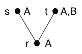
The labelling cannot be completely arbitrary. The relation \(\Vdash_\tau\) must satisfy a monotonicity condition, which says that if a label appears at a node, it appears at all descendants of that node. Formally, if \(c\Vdash_\tau X\), and \(c'\) is a descendant of \(c\), then \(c'\Vdash_\tau X\). Since we’ll be talking about descendants, let’s invent a notation: \(c\tl c'\) means that \(c'\) is a descendant of \(c\), that is, either \(c=c'\), or for some child \(c''\) of \(c\), \(c''\tl c'\). To remember this notation (which is not standard), when you look at \(c\tl c'\), think of the triangle as the subtree of \(\tau\) rooted at \(c\); that subtree contains \(c'\).
Kripke models don’t have to be trees in general, but finite trees suffice for discussion of IPL. The nodes are often called "possible worlds", and the forcing relation can be seen as describing what propositional variables are known to be true in a given world. The branching of the tree allows for different future possibilities, and the monotonicity condition ensures that our state of knowledge does not decrease with time. In the example above, we know that \(A\) is true at the root world, but we don’t know anything about \(B\). In all descendant worlds, we still know that \(A\) is true (that is, we don’t forget, and we don’t learn the opposite), and in one possible world, we learn that \(B\) is true. Here there is a single two-way branch, but trees can have arbitrary branching.
This possible-worlds metaphor can help us to remember the conditions on a Kripke model. The metaphor is interesting and possibly illuminating, but it isn’t necessary to use it in order to work with Kripke models; all we need are the mathematical definitions and their mathematical consequences.
We extend \(\Vdash_\tau\) to formulas using the following recursive definition. Pay special attention to the implication case, which is not like the others.
\(c\Vdash_\tau T \vee W\) iff \(c\Vdash_\tau T\) or \(c\Vdash_\tau W\);
\(c\Vdash_\tau T \wedge W\) iff \(c\Vdash_\tau T\) and \(c\Vdash_\tau W\);
\(c\Vdash_\tau T \ra W\) iff for all \(c'\) such that \(c\tl c'\), if \(c'\Vdash_\tau T\), then \(c'\Vdash_\tau W\);
\(c\Vdash_\tau\bot\) never holds.
Going back to the possible-worlds metaphor, what does it mean to know \(T \ra W\) in a world? We might not know anything about \(T\) or \(W\) in that world. But in a descendant world where we learn that \(T\) is true, \(W\) should also be true. Note that this allows for the possibility that we never learn that \(T\) is true. That is, the definition of \(c\Vdash_\tau T \ra W\) is satisfied if for all \(c'\) such that \(c\tl c'\), \(c'\Vdash_\tau T\) does not hold (we can write this as \(c'\nVdash_\tau T\)). This is true regardless of what we know or don’t know about \(W\).
As a consequence of the last two clauses of the last definition, and our intuitionistic definition of logical negation, \(\lnot T\) is forced in a world exactly when \(T\) is not forced in any descendant world. Formally, \(c\Vdash_\tau \lnot T\) if and only if for all \(c'\) such that \(c \tl c'\), \(c'\nVdash_\tau T\).
Consider the situation at a leaf \(\ell\) of \(\tau\). If we define a Boolean valuation by \(v(X)=1\) if and only if \(\ell\Vdash_\tau X\), then it is not hard to see that \(\ell\Vdash_\tau T\) if and only if \(\langle T \rangle_v=1\). So if the tree is a single node, we just have the Boolean notion of truth. It is the possibility of trees with more than one node that lets us create a notion of truth that corresponds to formulas provable in IPL.
It is also not hard to see (or prove by a simple induction on formulas) that monotonicity extends to formulas, that is, if a formula is true at a node, then it is true at all descendant nodes. Formally, if \(c\Vdash_\tau T\) and \(c \tl c'\), then \(c'\Vdash_\tau T\). The contrapositive of monotonicity will also be useful: if a formula is not true at a node, then it is not true at all ancestor nodes. Formally, if \(c'\nVdash_\tau T\) and \(c \tl c'\), then \(c\nVdash_\tau T\).
Now we can define the semantic notion of truth for a formula with respect to Kripke models, using the same idea as for the Boolean interpretation but substituting Kripke semantics. We define \(\Gamma\vDash_K T\) to mean that for all Kripke models \(\tau\) with root \(r\), and all forcing functions \(\Vdash_\tau\), whenever \(r\Vdash_\tau W\) for all \(W \in \Gamma\), \(r\Vdash_\tau T\) holds.
Soundness means that for all contexts \(\Gamma\) and all formulas \(T\), \(\Gamma\vdash_I T\) implies \(\Gamma\vDash_K T\). Soundness can be proved by induction on the proof tree. As an example of the case analysis, let us take the case where the rule applied at the root of the proof tree is \(\ra_I\). (The other cases are much easier, as implication is the case in the definition of \(\Vdash\) where the tree is actually taken into account.)
Suppose that \(T=V\ra W\) and the conclusion at the root of the proof tree is \(\Gamma\vdash_I V\ra W\). Then the premise of the application of the \(\ra_I\) rule is \(\Gamma,V\vdash W\). By the induction hypothesis applied to the proof tree of this premise (the whole proof tree with the root removed), \(\Gamma,V\vDash_K W\). This means that for any \(\tau\) with root \(r\) such that for all \(S\in\Gamma,V\), \(r\Vdash_\tau S\), we also have that \(r\Vdash_\tau W\). We need to show \(\Gamma\vDash_K V\ra W\). This means that for all \(\tau\) with root \(r\) and for all \(S\in\Gamma\), \(r\Vdash_\tau S\), we also have that for all \(c\) in \(\tau\), \(c\Vdash_\tau V\) implies \(c\Vdash_\tau W\). To show this, we note that if we have such a \(\tau\), then by monotonicity, for all \(S\in\Gamma\), \(c\Vdash_\tau S\). If also \(c\Vdash_\tau V\), then \(c\Vdash_\tau S\) for all \(S\in\Gamma,V\). We apply the inductive hypothesis to the tree \(\tau'\) rooted at \(c\), and conclude that \(c\Vdash_{\tau'} W\), from which it follows that \(c\Vdash_\tau W\), as required. You should check one of the other cases to see that it is in fact easier than this.
The contrapositive of soundness is: given a context \(\Gamma\) and a formula \(T\), \(\Gamma\nvDash_K T\) implies \(\Gamma\nvdash_I T\). When \(\Gamma\) is the empty context, this lets us prove that certain formulas that are provable in CPL are not provable in IPL. To demonstrate \(\Gamma\nvDash_K T\), we provide a Kripke model \(\tau\) with root \(r\), and show that \(r\nVdash_\tau T\).
(Is the contrapositive intuitionistically provable? Our metamathematics does not hesitate to use classical logic, but in this case, the implication is intuitionistically provable!)
Consider \(A \lor \lnot A\). The Kripke model \(\tau\) we use has a root \(r\) with one child \(s\).
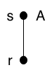
The relation \(\Vdash_\tau\) has \(s\Vdash_\tau A\) but does not relate \(r\) to anything. So \(r\nVdash_\tau A\). Since \(s\nVdash_\tau\bot\) but \(s\Vdash_\tau A\), \(s\nVdash_\tau A \ra \bot\), that is, \(s\nVDash_\tau \lnot A\). From this and \(r\tl s\), by the contrapositive of monotonicity, \(r\nVdash_\tau \lnot A\). Combining that with \(r\nVdash_\tau A\), we have \(r\nVdash_\tau A \lor \lnot A\), and therefore \(\nvDash_K A \lor \lnot A\). Finally, by the contrapositive of soundness, \(\nvdash_I A \lor \lnot A\).
Below are some exercises along the lines above. The first exercise asks you to write a Racket program to decide entailment in Kripke models. This will help to confirm the models in your answers to the rest of the exercises, but it won’t help you to understand why the models work for their intended purpose. For that, you need reasoning like in the previous paragraph.
A trace of the computation of the Racket program would suffice as justification, but it would not be very readable, and would likely include some parts which are unnecessary. It’s worth reviewing the tools we have for minimal justifications such as the one above. Monotonicity for formulas lets us take the conclusion that a given formula is true at a given tree node, and move it to descendants of that tree node. The contrapositive of monotonicity lets us take the conclusion that a given formula is not true at a given tree node, and move it to ancestors of that tree node (most usefully, to the root).
Since the conclusion we want is of the form \(r\nVdash_\tau T\), we can look carefully at the rules for \(r\Vdash_\tau T\) and list what must hold to make each one fail. For a node \(c\) in tree \(\tau\), we break things down by the main connective of the formula:
\(c\nVdash_\tau T \vee W\) iff both \(c\nVdash_\tau T\) and \(c\nVdash_\tau W\);
\(c\nVdash_\tau T \wedge W\) iff one of \(c\nVdash_\tau T\) and \(c\nVdash_\tau W\) holds (possibly both, but one is all that’s needed);
\(c\nVdash_\tau T \ra W\) iff there is some \(c'\) such that \(c\tl c'\), \(c'\Vdash_\tau T\), but \(c'\nVdash_\tau W\) (again, there may be many, but one is all that’s needed);
\(c\nVdash_\tau\bot\) always holds.
That gives us tools for justifying a Kripke model, but how do we construct one in the first place, given the formula we wish to show unprovable in IPL? This is more of an art (though there is an algorithm, as discussed below). One way to think about it is to anticipate the use of the tools of justification.
Let me illustrate with a plausible sequence resulting in the model above that shows that \(A \lor \lnot A\) is not provable. We start with just the root \(r\) as our model \(\tau\). That alone won’t suffice, since we know that a one-node model just defines a Boolean valuation, and our formula is satisfied by all Boolean valuations. Our goal is to eventually show \(r\nVdash_\tau A \lor \lnot A\) (for the \(\tau\) we construct).
Since this is a disjunction, we need to show that both of the following hold: \(r\nVdash_\tau A\) and \(r\nVdash_\tau \lnot A\). For the first one, we just make sure that \(r\) does not force \(A\), by not labelling it with \(A\). The second one requires \(r\nVdash_\tau A \ra \bot\). To show this, we need a descendant \(s\) of \(r\) for which \(s\Vdash_\tau A\) and \(s\nVdash_\tau \bot\). The second always holds, and for the first, we must label \(s\) with \(A\).
That seems to cover everything, though in general we might need to check that we haven’t broken previous subgoals while adding something to the model. This example doesn’t require branching in the tree, but keep that in mind.
Exercise 7: Write a Racket program to validate a Kripke model with respect to a formula. You can use an S-expression representation: a KM is a list containing the root symbol, a list of variables forced at the root, and a KM for each child of the root. Include a function valid? that consumes a KM and produces #t if and only if the model is valid (satisfies the monotonicity condition), and a function forced-at? that consumes a valid KM and a formula and produces #t if and only if the formula is forced at the root of the KM. Don’t worry too much about efficiency, as the models and formulas will tend to be small. \(\blacksquare\)
\(\lnot \lnot A \ra A\)
\(\lnot (A \land B) \ra \lnot A \lor \lnot B\)
\(((A \ra B) \ra A) \ra A\)
\((A \ra B) \lor (B \ra A)\)
Completeness (\(\Gamma\vDash_K T\) implies \(\Gamma\vdash_I T\)) is also provable, but it is more complicated. The most elegant proof for IPL that I’ve seen is an adaptation of one of the elegant nonconstructive proofs for CPL. One constructive way of proving completeness is via a proof search procedure using what are called tableaux. If the procedure fails to find a proof, the search tree can be converted into a Kripke model demonstrating unprovability. This is an algorithm in service of a metamathematical theorem, but there is a lot of interest in algorithms on formulas, usually in the related context of the satisfiability problem, which can be summarized as "Does there exist a valuation making a given formula true?" Practical solutions have many applications, and an entirely separate course could be built on them.
Even a nonconstructive proof for completeness will allow us to construct an algorithm to decide whether or not a formula is provable in IPL. In parallel, start generating all possible proof trees and all possible Kripke models using the variables of the formula. As you generate each one, check whether it proves the formula or whether it shows the formula cannot be proved, respectively. One of the two parallel streams will succeed.
This is not a very good algorithm. Better ones exist, but they are still not particularly efficient in the worst case, and there is complexity-theoretic evidence that the problem is strictly harder for IPL than for CPL.
There is plenty more to say about IPL, but your patience is probably limited, so let me just mention one possibly useful topic before moving on to predicate logic. Glivenko proved two theorems about IPL in 1929. The first is that a negated formula (one that has negation as its root connective) can be proved in IPL if and only if it can be proved in CPL. Formally, \(\vdash_I \lnot T\) if and only if \(\vdash_C \lnot T\). The second is that a formula can be proved in CPL if and only if its double negation can be proved in IPL. Formally, \(\vdash_C T\) if and only if \(\vdash_I \lnot \lnot T\).
Challenge: prove Glivenko’s two theorems using completeness for IPL.
\(\lnot \lnot (A \lor \lnot A)\)
\(\lnot \lnot (\lnot \lnot A \ra A)\)
In effect, CPL can be embedded into IPL, so we do not lose anything in terms of provability by choosing to work with intuitionistic logic. Similar translations (though a bit more complicated) are available for predicate logic.
2.10 Summary of rules for intuitionistic propositional logic
These are collected from above for reference.
Variables:
\[\ir{(\mbox{Var})}{}{\Gamma, x:X\vdash x \Ra X}\]
Implication:
\[\ir{(\ra_I)}{\Gamma,x:T\vdash t \La W}{\Gamma\vdash \la x.t \La T\ra W}\]
\[\ir{(\ra_E)}{\Gamma\vdash f \Ra T\ra W ~~~ \Gamma\vdash a \La T}{\Gamma\vdash f~a \Ra W} \\\]
The turn rule:
\[\ir{(\mbox{Turn})}{\Gamma\vdash t \Ra T' ~~~~ T \equiv T'}{\Gamma\vdash t\La T}\]
Annotation:
\[\ir{(\mbox{Ann})}{\Gamma\vdash t\La T}{\Gamma\vdash (t:T)\Ra T}\]
Conjunction:
\[\ir{(\land_I)}{\Gamma\vdash t\La T ~~\Gamma\vdash w\La W} {\Gamma\vdash\land_\mathit{intro}~t~w\La T\land W}\]
\[\ir{(\land_{E0})}{\Gamma\vdash v\Ra T\land W} {\Gamma\vdash\land_\mathit{elim0}~v\Ra T} ~~ \ir{(\land_{E1})}{\Gamma\vdash v\Ra T\land W} {\Gamma\vdash\land_\mathit{elim1}~v\Ra W}\]
Disjunction:
\[\ir{(\lor_{I0})}{\Gamma\vdash t\La T} {\Gamma\vdash\lor_\mathit{intro0}~t\La T\lor W} ~~ \ir{(\lor_{I1})}{\Gamma\vdash w\La W} {\Gamma\vdash\lor_\mathit{intro1}~w\La T\lor W}\]
\[\ir{(\lor_E)} {\Gamma\vdash d\Ra T\lor W ~~~~ \Gamma\vdash f\La T\ra V ~~~~\Gamma\vdash g\La W\ra V} {\Gamma\vdash\lor_\mathit{elim}~d~f~g\La V}\]
Bottom elimination:
\[\ir{(\bot_{E})}{\Gamma\vdash t\La\bot} {\Gamma\vdash \bot_\mathit{elim}~t\La T}\]
Negation: \(\lnot T\) is \(T \ra \bot\).