Hybrid Symbolic-Numeric Integration in Maple
Keith O. Geddes
Symbolic Computation Group, School of Computer Science
University of Waterloo, Waterloo, ON, N2L 3G1, Canada
Abstract
The Maple scientific computation environment supports both symbolic and numeric mathematical computation. In this presentation, the paradigm of hybrid symbolic-numeric computation is employed to achieve an enhanced level of computational power. The overall strategy is to apply an appropriate combination of symbolic mathematical analysis and numerical computation.
The hybrid symbolic-numeric methods illustrated here are part of an automated numerical integration strategy [Geddes86, Geddes92] implemented in Maple for the numerical evaluation of definite integrals. In particular, symbolic analysis techniques are used to deal with integrand singularities.
Example 1: Finite and Infinite Interval of Integration
| > |
 |
| > |
 |

| > |
 |
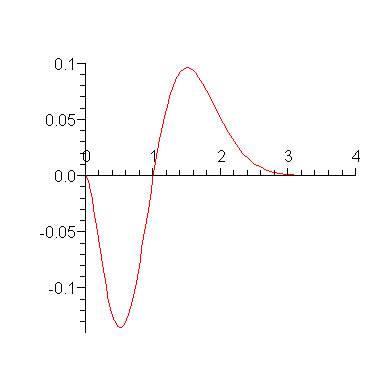
Form the integral on  and attempt to evaluate in symbolic mode.
| > |
 |

The integral does not evaluate in symbolic mode. Apply direct numerical integration (at standard precision).
| > |
 |

The above result was computed by invoking compiled NAG routines.
Or at higher precision:
| > |
 |

Notice from the graph that the integral on  will have approximately the same numerical value as the above result on
  .
.
Curiously, for the infinite integral a closed form expression can be obtained!
| > |
 |

| > |
 |

| > |
 |

Or, we may apply direct numerical integration to the infinite integral.
| > |
 |

Note: Numerical evaluation of the exact formula loses some precision. The result from numerical integration is correct to 10 significant digits.
Example 2: Logarithmic singularity at left endpoint
| > |
 |
| > |
 |

| > |
 |
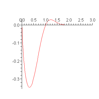
Form the integral on  , attempt symbolic evaluation, and apply numerical integration.
| > |
 |

| > |
 |

Evaluating numerically to  digits yields the following result.
| > |
 |

Note that
the integrand has a logarithmic singularity at  as the following series expansion shows.
| > |
 |

The hybrid symbolic-numeric technique includes the concept of term-by-term integration of such a series expansion.
Example 3: Subtracting off a singularity
| > |
 |
| > |
 |
| > |
 |

Note that the graph of this integrand goes to  at
at  . However, this is an integrable singularity: it behaves like
  near
near  .
.
| > |
 |
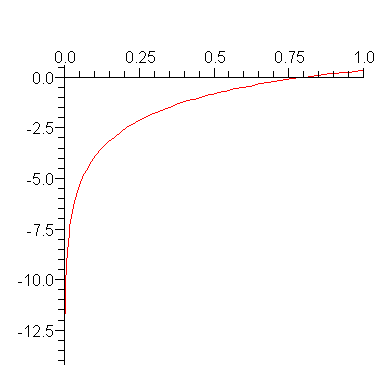
Note: The technique of subtracting off a singularity illustrated below, takes place automatically within Maple's numerical integration routines.
Suppose it is desired to compute the result to  digits of accuracy. The generalized series expansion of
  at
at  takes the following form.
| > |
 |
| > |
 |

The non-regular part is
| > |
 |

The new expression
| > |
 |

is analytic on the interval ![[0, 1]](images/NumInt_59.gif) . Thus it can be integrated easily by the default numerical integration method.
. Thus it can be integrated easily by the default numerical integration method.
| > |
 |

Integrating  is easy because it has the indefinite integral
| > |
 |

and its definite integral can therefore be computed symbolically:
| > |
 |

Finally, summing the two values, we obtain the value for the original definite integration problem.
| > |
 |

Example 4: Algebraic transformation of variables
| > |
 |
| > |
 |

| > |
 |

Note: The change of variables illustrated below takes place automatically within Maple's numerical integration routines.
The generalized series expansion of the integrand  at
at  is of the form
| > |
 |

Applying the change of variables  yields
| > |
 |

The new integrand is analytic on the interval of integration. Therefore it can be integrated easily by the default numerical integration method, even at high accuracy. Suppose that the result is desired to  digits of accuracy:
| > |
 |

Example 5: Integrating a series term-by-term
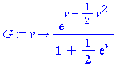
| > |
 |
| > |
 |
| > |
 |
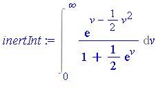
Note: The development of the integrand in a generalized series expansion and its integration term-by-term as illustrated below takes place automatically within Maple's numerical integration routines.
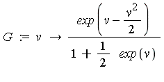
Suppose it is desired to compute the integral to  digits of accuracy. First, the interval of integration is split into
  and
and  . For the finite interval, the default numerical integration method has no difficulty.
| > |
 |

| > |
 |

For the infinite interval, the change of variables  transforms the problem into the following new integration problem.
| > |
 |
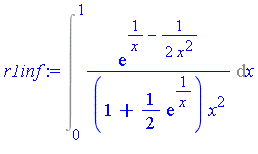
Let the integrand appearing here be named  . The first few terms of the generalized series expansion of
  are as follows.
| > |
 |
| > |
 |
| > |
 |


Note that  is a series in increasing powers of
  . Maple's symbolic integrator determines that the first two terms of
  have the following indefinite integrals.
| > |
![terms := [seq(simplify(op(i, s), symbolic), i = 1 .. n)]; -1](images/NumInt_111.gif) |
| > |
 |

| > |
 |

Similarly, the integral of each term can be computed symbolically. If we compute the definite integral over [0, 0.25] of the successive terms of the generalized series expansion of  , we find that the successive values are as follows. For the numerical evaluation of the symbolic formula for each term, and for the addition of the terms to get an accurate floating point result, it is generally necessary to set the working precision higher for this stage of the computation.
| > |
 |
| > |
 |


Clearly, the series representation is converging reasonably quickly on this interval (the magnitude of successive terms is decreasing at a good rate).
To obtain a numerical result accurate to 20 digits, it is necessary to sum more than six terms of the series as can be seen from the magnitude of the terms above. For this example, 20 terms is more than necessary.
| > |
s := `evalf/int/genseries`(g, x, n): |
| > |
terms := [seq(simplify(op(i,s),symbolic), i=1..n)]: |
The following loop adds successive terms until the magnitude of the terms becomes negligible for 20 digit accuracy.
| > |
t := evalf( int(terms[1], x=0..0.25) ): val := t: |
| > |
for i from 2 to n while abs(t/val) > epsilon do
t := evalf( int(terms[i], x=0..0.25) );
val := val + t
end do: |
| > |
number_of_terms := i-1; |

We now have the following result for the integral of  over [0, 0.25] .
| > |
 |
| > |
 |

For the remaining interval [0.25, 1] , ordinary numerical integration methods encounter no difficulties because there are no nearby singularities.
| > |
 |

Add these two values to get the value of the integral  .
.
| > |
 |

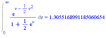
Finally, we have obtained the answer for the original integration problem.
| > |
 |
Multidimensional Numerical Integration
In Maple, one can always express a multiple integral using nested one-dimensional integrals. For example:
| > |
 |
| > |
 |
| > |
 |

In older versions (prior to Maple 8), one could invoke the  command on a multiple integral such as above; however, the only solution method was to invoke, recursively, one-dimensional numerical integration methods. This was an inefficient approach to numerical multiple integration problems which would succeed only on the simplest problems.
In more recent versions, specific methods for numerical multiple integration were introduced. The following command automatically invokes a compiled C routine to compute the multiple integral.
| > |
 |

It is also possible to express multiple integrals using a special list syntax, which is sometimes more convenient.
Special (list) syntax for multiple integrals
A numerical multiple integration problem can be specified in a natural way using nested one-dimensional integrals, as shown above. In 1-D input notation, this takes the general form:


where the integrand  depends on
  . Such a problem can also be specified using the following special multiple integration notation with a list as the second argument:
 .
.
Additional optional arguments can be stated just as in the case of one-dimensional integration. Also as in one-dimensional integration, the integrand  can be specified as a procedure in which case the second argument must be a list of ranges:
  . Whether a multiple integration problem is stated using nested integrals or using the list notation, the arguments are extracted so as to invoke the same numerical multiple integration routines. See the help page
  for further details and examples.
Example 6
Numerical evaluation of the triple integral given above, expressed in 1-D input notation, takes the following form (again using nested one-dimensional integrals):
| > |

 |

Using the list syntax, this same computation can be expressed as follows:
| > |
 |

Example 7
| > |
 |
| > |
 |
| > |
 |


| > |

 |

The same computation can be expressed using the list syntax as follows.
| > |
 |

It is important to note that expressing the computation in either form leads to the same numerical multiple integration routines being invoked.
Example 8
When low accuracy is sufficient, the Monte Carlo method may be used. For example, suppose that we wish to compute the following multiple integral.
| > |
 |
| > |
![Int(Int(Int(Int(Int(Int(h, x[1] = -1 .. 1), x[2] = -1 .. 1), x[3] = -1 .. 1), x[4] = -1 .. 1), x[5] = -1 .. 1), x[6] = -1 .. 1); -1](images/NumInt_168.gif) |
where
| > |
![h := 1/(2+sin(Pi*sqrt(87)*(x[1]+x[2]+x[3]+x[4]+x[5]+x[6]))); -1](images/NumInt_169.gif) |
The computation can be expressed as follows.
Only trust about  digits because the requested accuracy was
  . (The Monte Carlo method is only appropriate for computing a few digits of accuracy.)
| > |
 |

References
[Geddes86] K.O. Geddes, Numerical integration in a symbolic context. Proceedings of SYMSAC'86, B.W. Char (ed.), ACM Press, New York, 1986, pp. 185-191.
[Geddes92] K.O. Geddes and G.J. Fee, Hybrid symbolic-numeric integration in Maple. Proceedings of ISSAC'92, P.S. Wang (ed.), ACM Press, New York, 1992, pp. 36-41.


![]() and attempt to evaluate in symbolic mode.
and attempt to evaluate in symbolic mode. 

![]()
![]()
![]() will have approximately the same numerical value as the above result on
will have approximately the same numerical value as the above result on ![]() .
. 


![]()
![]()


 transforms the problem into the following new integration problem.


![Int(Int(Int(Int(Int(Int(h, x[1] = -1 .. 1), x[2] = -1 .. 1), x[3] = -1 .. 1), x[4] = -1 .. 1), x[5] = -1 .. 1), x[6] = -1 .. 1); -1](images/NumInt_168.gif)
![h := 1/(2+sin(Pi*sqrt(87)*(x[1]+x[2]+x[3]+x[4]+x[5]+x[6]))); -1](images/NumInt_169.gif)
 . (The Monte Carlo method is only appropriate for computing a few digits of accuracy.)