Hybrid Symbolic-Numeric Integration in Multiple Dimensions via Tensor-Product Series
Orlando A. Carvajal
Frederick W. Chapman
Keith O. Geddes
Symbolic Computation Group, School of Computer Science
University of Waterloo, Waterloo, ON, N2L 3G1, Canada
Abstract
We present a new hybrid symbolic-numeric method for the fast and accurate evaluation of definite integrals in multiple dimensions. This method is well-suited for two classes of problems: (1) analytic integrands over general regions in two dimensions, and (2) families of analytic integrands with special algebraic structure over hyperrectangular regions in higher dimensions.
The algebraic theory of multivariate interpolation via natural tensor-product series was developed in the doctoral thesis by Chapman, who named this broad new scheme of bilinear series expansions ”Geddes series” in honour of his thesis supervisor. This paper describes an efficient adaptive algorithm for generating bilinear series of Geddes-Newton type and explores applications of this algorithm to multiple integration. We will present test results demonstrating that our new adaptive integration algorithm is effective both in high dimensions and with high accuracy. For example, our Maple implementation of the algorithm has successfully computed nontrivial integrals with hundreds of dimensions to 10-digit accuracy, each in under 3 minutes on a desktop computer.
Current numerical multiple integration methods either become very slow or yield only low accuracy in high dimensions, due to the necessity to sample the integrand at a very large number of points. Our approach overcomes this difficulty by using a Geddes-Newton series with a modest number of terms to construct an accurate tensor-product approximation of the integrand. The partial separation of variables achieved in this way reduces the original integral to a manageable bilinear combination of integrals of essentially half the original dimension. We continue halving the dimensions recursively until obtaining one-dimensional integrals, which are then computed by standard numeric or symbolic techniques.
Introduction
The hybrid symbolic-numeric method presented in this paper is well-suited for two classes of integration problems:
- . analytic integrands over general regions in two dimensions, and
- . families of analytic integrands with special algebraic structure over hyperrectangular regions in higher dimensions.
Summary of the Method
- The method is based on recursive dimension-halving via separation of variables.
- Multidimensional integrals are reduced to one-dimensional integrals using Geddes-Newton series expansions to generate accurate tensor-product approximations of the integrand.
- Test results show that our new adaptive integration algorithm is effective both with high accuracy and in high dimensions.
Tensor-Product Series
Tensor Products
- A tensor product is a finite sum of terms where each term is a product of univariate functions:
 = Sum(g[i](x)*h[i](y), i = 1 .. n)](images/MultiInt_1.gif)
- There are many examples in mathematics:


- The rank of a tensor product is the minimum number of terms among all the equivalent representations.
- It is a natural tensor product when the factors of each term can be derived from the original function by a finite linear combination of linear functionals.
The Splitting Operator
- For a bivariate function
 and a point
  where
where  , the splitting operator
 ![Upsilon[a, b]](images/MultiInt_8.gif) is defined by
is defined by
![Upsilon[a, b]*f(x, y) = f(x, b)*f(a, y)/f(a, b)](images/MultiInt_9.gif) .
.
- The point
 is called a splitting point.
- Note:
![Upsilon[a, b]](images/MultiInt_11.gif) splits
splits  into a rank-one tensor product.
![Upsilon[a, b]*f(x, y)](images/MultiInt_13.gif) interpolates
interpolates  on the lines
  and
and  , which means that
 ![Upsilon[a, b]*`≡`(f(a, y), f(a, y))](images/MultiInt_17.gif) and
and ![Upsilon[a, b]*`≡`(f(x, b), f(x, b))](images/MultiInt_18.gif) .
.
- These properties allow us to generate a natural tensor-product series simply by iterating the splitting operator while varying the choice of splitting point.
Geddes-Newton Series Expansions
- Not every bivariate function
 can be expressed as a tensor product of finite rank.
- For an approximation in
![R = Typesetting:-delayCrossProduct([a, b], [c, d])](images/MultiInt_20.gif) where
where  is continuous, we can uniformly approximate
  by a rank-
 tensor product:
 = Sum(g[i](x)*h[i](y), i = 1 .. n)](images/MultiInt_24.gif)
- Define the
 remainder :
 ![r[n] = f-s[n]](images/MultiInt_26.gif) .
.
- The following simple algorithm generates a natural tensor-product series expansion
![s[n]](images/MultiInt_27.gif) of a given function
of a given function  on
on  .
.
Algorithm NTPS
- . Set
![r[0] := f](images/MultiInt_30.gif) and initialize
and initialize  .
.
- . While
![delta < LinearAlgebra:-Norm(r[i-1], infinity)](images/MultiInt_32.gif) , iterate the following:
, iterate the following:
- ) Choose
![`in`(a[i], b[i], R)](images/MultiInt_33.gif) with
with ) = LinearAlgebra:-Norm(r[i-1], infinity)](images/MultiInt_34.gif) .
.
- ) Let
![r[i] := r[i-1]-Upsilon[a[i], b[i]]*r[i-1]](images/MultiInt_35.gif) and
and  .
.
- . Let
 and return
 ![s[n] := f-r[n]](images/MultiInt_38.gif) to approximate
to approximate  with uniform error
 ![LinearAlgebra:-Norm(r[n], infinity) <= delta](images/MultiInt_40.gif) on
on  .
.
- Refining terminology introduced by Chapman in his doctoral thesis, we call
![s[n]](images/MultiInt_42.gif) the Geddes-Newton series expansion of
the Geddes-Newton series expansion of  to
to  terms with respect to the splitting points
 ![({a[i], b[i]})[i = 1]^n](images/MultiInt_45.gif) .
.
Example 1
Consider the following function on ![Typesetting:-delayCrossProduct([0, 1], [0, 1])](images/MultiInt_46.gif) :
:

The Geddes-Newton series to 3 terms is as follows, where the splitting points are  for
for  :
:
 = Sum(c[i]*g[i](x)*h[i](y), i = 1 .. 3)](images/MultiInt_50.gif)
where
![c[1] = -.884017](images/MultiInt_51.gif)
 = exp(x^2)*cos(x+1)](images/MultiInt_52.gif)
 = exp(y^2)*cos(y+1)](images/MultiInt_53.gif)
![c[2] = .794868](images/MultiInt_54.gif)
 = cos(x)+.477636*exp(x^2)*cos(x+1)](images/MultiInt_55.gif)
 = cos(y)+.477636*exp(y^2)*cos(y+1)](images/MultiInt_56.gif)
![c[3] = -9.83284](images/MultiInt_57.gif)
 = exp(.379870*x^2)*cos(x+.616336)-.356576*exp(x^2)*cos(x+1)-.623342*cos(x)](images/MultiInt_58.gif)
 = exp(.379870*x^2)*cos(x+.616336)-.356576*exp(x^2)*cos(x+1)-.623342*cos(x)](images/MultiInt_59.gif)
 = exp(.379870*x^2)*cos(x+.616336)-.356576*exp(x^2)*cos(x+1)-.623342*cos(x)](images/MultiInt_60.gif)
 = exp(.379870*y^2)*cos(y+.616336)-.356576*exp(y^2)*cos(y+1)-.623342*cos(y)](images/MultiInt_61.gif)
 = exp(.379870*y^2)*cos(y+.616336)-.356576*exp(y^2)*cos(y+1)-.623342*cos(y)](images/MultiInt_62.gif)
 = exp(.379870*y^2)*cos(y+.616336)-.356576*exp(y^2)*cos(y+1)-.623342*cos(y)](images/MultiInt_63.gif)
Observations
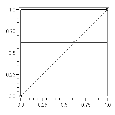
- The splitting points in Example 1 are all located on the diagonal
 of the unit square, as illustrated in the following figure.
- Note:
](images/MultiInt_66.gif) agrees exactly with
agrees exactly with  at all points on the horizontal and vertical lines through the three splitting points!
- With this strong interpolating property, even with only three splitting points we find that the maximum error over the unit square satisfies:
![`≈`(LinearAlgebra:-Norm(f-s[3], infinity), `*`(3.0, `^`(10, -3)))](images/MultiInt_68.gif) .
.
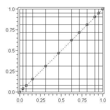
- If we request a series accurate to 15 digits for the function
 defined in Example 1, we find that only 12 terms are required (i.e., 12 splitting points). In other words,
 ![LinearAlgebra:-Norm(f-s[12], infinity) < `*`(5.0, `^`(10, -15))](images/MultiInt_70.gif) .
.
- The distribution of the 12 splitting points for this particular function is illustrated in the following figure.
Convergence of the Series
- Note similarities with the case of univariate polynomial interpolation via the Newton interpolation series.
- In both cases, addition of a new term in the series corresponds to the addition of a new interpolation point.
- However, in the case of Geddes-Newton series, the interpolation property holds not only at the new point but at all points on two lines passing through that point.
- Intuitively, for any function
 which is continuous in the unit square
  , if the splitting points are dense along the diagonal then it is reasonable to expect that
 ![s[n]](images/MultiInt_74.gif) might converge uniformly to
might converge uniformly to  on
on  as
as  .
.
- In other words, by choosing well distributed splitting points on the diagonal, we can cover the whole unit square with small grid cells. Recall: The remainder
![r[n]](images/MultiInt_78.gif) vanishes on the boundary of each cell .
vanishes on the boundary of each cell .
- Formal convergence results will appear in a separate paper.
A Brief Glance at Proof Technique
- The easiest case is when
 is analytic in a sufficiently large region.
- The convergence theorem and its proof are similar to the classical case where
 is a function of a single complex variable and
 ](images/MultiInt_81.gif) denotes the interpolating polynomial.
denotes the interpolating polynomial.
- Recall the univariate case (Ref: P.J. Davis, Interpolation and Approximation), as summarized below.
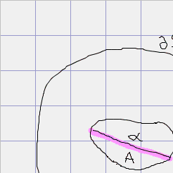
- Basic tool: A contour integral representation of
](images/MultiInt_82.gif) .
.
- Let
 be analytic on be analytic on  and suppose that the interpolation points satisfy and suppose that the interpolation points satisfy ![`in`(a[i], `⊂`(A, S))](images/MultiInt_85.gif) . .
- Let
](images/MultiInt_86.gif) be the polynomial interpolating be the polynomial interpolating  at points at points ![{a[i]}](images/MultiInt_88.gif) . .
 , ,  . .
- Conclusion: If
 then then
![limit(LinearAlgebra:-Norm(f-s[n], A), n = infinity) = 0](images/MultiInt_95.gif) . .
|
|
- For our case, we consider a bivariate function
 of two complex variables and
 ](images/MultiInt_98.gif) denotes the Geddes-Newton series expansion of
denotes the Geddes-Newton series expansion of  to
to  terms with respect to the splitting points
 ![{a[i], b[i]}](images/MultiInt_101.gif) .
.
- We derive a contour integration formula for the remainder
![r[n] = f-s[n]](images/MultiInt_106.gif) :
: 


- Here,
 = product(w-a[k], k = 1 .. n)](images/MultiInt_111.gif) and
and  = product(z-b[k], k = 1 .. n)](images/MultiInt_112.gif) .
.
- Then we can conclude that
![LinearAlgebra:-Norm(r[n], Typesetting:-delayCrossProduct(A, B)) <= M*gamma^n*LinearAlgebra:-Norm(r[n], Typesetting:-delayCrossProduct(`∂`(S), `∂`(T)))](images/MultiInt_113.gif) where the constant
where the constant  depends on the geometry, and
  depends on separation constants (like before).
- If
 and if the
  boundary constant satisfies
![LinearAlgebra:-Norm(r[n], Typesetting:-delayCrossProduct(`∂`(S), `∂`(T))) = o(gamma^(-n))](images/MultiInt_118.gif) as
as  then
then ![limit(LinearAlgebra:-Norm(f-s[n], Typesetting:-delayCrossProduct(A, B)), n = infinity) = 0](images/MultiInt_120.gif) .
.
Integration in Two Dimensions
- The given integration problem is
 .
.
- Approximate the integrand
)](images/MultiInt_122.gif) and then integrate:
and then integrate:  .
.
- We replace the calculation of one integral in two dimensions by
 integrals each in one dimension:

- The effectiveness of this scheme relies on the following facts:
- we have good methods to compute one-dimensional integrals, either in numerical mode or (advantageous in certain situations) symbolic mode
- the number of terms
 is of modest size (for many integrands of interest) due to the power of this particular interpolation scheme
- we exploit symmetry and apply efficient linear algebra computations, as discussed next
Transformation to Canonical 2-D Integral
- An integral with non-constant limits can be converted to a new integral with constant limits via a change of variables.

using the change of variables:
 ;
; 
- Therefore limit attention to integrals on the unit square.
- Making the integrand symmetric: For an integral on the unit square, we can always make the integrand symmetric, meaning
 .
.
- Namely,
![f = f[S]+f[A]](images/MultiInt_131.gif) (symmetric part + anti-symmetric part) where
(symmetric part + anti-symmetric part) where
 = `*`(f(x, y)+f(y, x), 1/2)](images/MultiInt_132.gif) ;
; 
- Integral of
![f[A]](images/MultiInt_134.gif) over the unit square is
over the unit square is  , which gives us:
, y = 0 .. 1), x = 0 .. 1)](images/MultiInt_136.gif) .
.
- Therefore we always have a symmetric integrand on the unit square.
Example 2
Consider the double integral

Applying the change of variables to transform to the unit square, and then applying symmetrization, yields the new problem:

where


Result of computation:
- Geddes-Newton series for
 was computed to 3 terms
- The series was integrated (applying one-dimensional quadratures)
- Computed result: 0.385433
- Result is correct to 5 significant digits (with only 3 terms)
Linear Algebra Formulation
- An efficient implementation is achieved by exploiting symmetry.
- The series resulting from our algorithm has the algebraic form:
 = Sum(c[i]*(Sum(k[i, j]*f(x, b[j]), j = 1 .. i))*(Sum(l[i, j]*f(a[j], y), j = 1 .. i)), i = 1 .. n)](images/MultiInt_142.gif)
where ![c[i], k[i, j], l[i, j] <> 0](images/MultiInt_143.gif) are real-valued constants, and
are real-valued constants, and ![a[i], b[i]](images/MultiInt_144.gif) is the splitting point used in the
is the splitting point used in the  iteration.
- Note that
![{a[i]} = {b[i]}](images/MultiInt_146.gif) .
.
- Represent the series using matrices and vectors as
 = V(x)^T*L^T*P*D*L*V(y)](images/MultiInt_147.gif)
where
 is the column vector of dimension
  with elements
 ![f(x, a[i])](images/MultiInt_150.gif)
 is an
is an  diagonal matrix with elements
 ![c[i] = 1/r[i-1](a[i], b[i])](images/MultiInt_153.gif)
 is a permutation matrix (identity matrix if splitting points all on diagonal)
![L = [l[i, j]]](images/MultiInt_155.gif) is an
is an  unit lower triangular matrix.
- Benefits of the matrix-vector representation:
- The cost of evaluating
![s[n]](images/MultiInt_157.gif) and
and ![r[n]](images/MultiInt_158.gif) is reduced from
is reduced from  to
to  evaluations of the original function
  .
.
- The factors can be computed by exploiting efficient linear algebra operations for matrix-vector multiplication and inner product.
- We only need to perform
 one-dimensional integrations of cross-sections of the original function:
 ![f(x, a[i])](images/MultiInt_163.gif) for
for  .
.
- The net effect: Nearly all the processing time is spent evaluating the integrand, which is as desired.
Computational Results in 2-D
The results in the following table are for the 2-D integral:

Tol
|
Time
|
Result
|
Pts
|
RelErr
|

|
0.3
|
0.069551393139
|
15
|

|

|
3.7
|
0.06955139313890799
|
21
|

|

|
5.3
|
0.0695513931389079901727
|
26
|

|

|
7.2
|
0.069551393138907990172712980
|
33
|

|

|
14.2
|
0.06955139313890799017271297964487
|
38
|

|
- Tol = requested accuracy tolerance
- Time = CPU time in seconds
- Result = computed value of the integral (to the number of digits requested)
- Pts = number of splitting points
- RelErr = relative error, compared with an accurate reference value
Integration in High Dimensions
- We have adapted our two-dimensional method to the case of
 -dimensional integrands
  which fit either of the following function patterns:

 .
.
- Can generate tensor-product approximations of such functions over the unit hypercube

- We call the method the Deconstruction / Approximation / Reconstruction Technique (DART).
The steps of DART
- . Deconstruction: Deconstruct
 to obtain a bivariate function
 +b)](images/MultiInt_182.gif) or
or *(at+b))](images/MultiInt_183.gif) .
.
- . Approximation: Approximate the symmetric function
 by a rank-
 tensor-product series
 ![s[n]](images/MultiInt_186.gif) in two variables on the unit square
in two variables on the unit square ![([0, 1])^2](images/MultiInt_187.gif) .
.
- . Reconstruction: By a change of variables, reconstruct the original function
 from
from  and produce a
  -variable tensor-product approximation
 ![S[n]](images/MultiInt_191.gif) of
of  on
on![([0, 1])^d](images/MultiInt_193.gif) from the bivariate approximation
from the bivariate approximation ![s[n]](images/MultiInt_194.gif) of
of  on
on ![([0, 1])^2](images/MultiInt_196.gif) .
.
Computational Results in High Dimensions
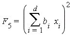
The results below are for the following families of  -dimensional integrands:
Note: ![F[5]](images/MultiInt_207.gif) and
and ![F[6]](images/MultiInt_208.gif) contain coefficients
contain coefficients ![b[i]](images/MultiInt_209.gif) which were assigned non-zero integer values in the range
which were assigned non-zero integer values in the range 
Here, the region of integration is the unit  -cube:
 ![`in`(x[i], [0, 1])](images/MultiInt_212.gif) for all
for all  , and the requested accuracy tolerance is fixed at
  .
.
Fcn
|
Dim
|
Time
|
Result
|
RelErr
|

|

|

|

|

|
![F[6]](images/MultiInt_220.gif)
|

|

|

|

|
![F[7]](images/MultiInt_225.gif)
|

|

|

|

|
![F[16]](images/MultiInt_230.gif)
|

|

|

|

|
![F[17]](images/MultiInt_235.gif)
|

|

|

|

|
![F[18]](images/MultiInt_240.gif)
|

|

|

|

|
![F[19]](images/MultiInt_245.gif)
|

|

|

|

|
![F[22]](images/MultiInt_250.gif)
|

|

|

|

|
- Fcn = the integrand function
- Dim = the dimension
 for that integrand;
  was chosen based on the criterion that for the given integrand, dimension
  would require > 3 min
- Time = CPU time in seconds
- Result = computed value of the integral (to the number of digits requested)
- RelErr = relative error, compared with an accurate reference value
References
O.A. Carvajal, A New Hybrid Symbolic-Numeric Method for Multiple Integration Based on Tensor-Product Series. Master's thesis, University of Waterloo, Waterloo, Ontario, Canada, 2004.
O.A. Carvajal, F.W. Chapman and K.O. Geddes, Hybrid symbolic-numeric integration in multiple dimensions via tensor-product series. Proceedings of ISSAC'05, Manuel Kauers (ed.), ACM Press, New York, 2005, pp. 84-91.
F.W. Chapman, Generalized Orthogonal Series for Natural Tensor Product Interpolation. Ph.D thesis, University of Waterloo, Waterloo, Ontario, Canada, 2003.
P.J. Davis, Interpolation and Approximation. Blaisdell, New York, 1963.
D.H. Thomas, A natural tensor product interpolation formula and the pseudoinverse of a matrix. Linear Algebra and Its Applications, 13 (3), 1976, pp. 239-250.
 = Sum(g[i](x)*h[i](y), i = 1 .. n)](images/MultiInt_1.gif)
![]()
![]()
![]()
 and a point
  where
where  , the splitting operator
 ![Upsilon[a, b]](images/MultiInt_8.gif) is defined by
is defined by
![Upsilon[a, b]*f(x, y) = f(x, b)*f(a, y)/f(a, b)](images/MultiInt_9.gif) .
.
 is called a splitting point.
![Upsilon[a, b]](images/MultiInt_11.gif) splits
splits  into a rank-one tensor product.
![Upsilon[a, b]*f(x, y)](images/MultiInt_13.gif) interpolates
interpolates  on the lines
  and
and  , which means that
 ![Upsilon[a, b]*`≡`(f(a, y), f(a, y))](images/MultiInt_17.gif) and
and ![Upsilon[a, b]*`≡`(f(x, b), f(x, b))](images/MultiInt_18.gif) .
.
 can be expressed as a tensor product of finite rank.
![R = Typesetting:-delayCrossProduct([a, b], [c, d])](images/MultiInt_20.gif) where
where  is continuous, we can uniformly approximate
  by a rank-
 tensor product:
 remainder :
 ![r[n] = f-s[n]](images/MultiInt_26.gif) .
.![s[n]](images/MultiInt_27.gif) of a given function
of a given function  on
on  .
.
![r[0] := f](images/MultiInt_30.gif) and initialize
and initialize  .
.![delta < LinearAlgebra:-Norm(r[i-1], infinity)](images/MultiInt_32.gif) , iterate the following:
, iterate the following:![`in`(a[i], b[i], R)](images/MultiInt_33.gif) with
with ) = LinearAlgebra:-Norm(r[i-1], infinity)](images/MultiInt_34.gif) .
.![r[i] := r[i-1]-Upsilon[a[i], b[i]]*r[i-1]](images/MultiInt_35.gif) and
and  .
. and return
 ![s[n] := f-r[n]](images/MultiInt_38.gif) to approximate
to approximate  with uniform error
 ![LinearAlgebra:-Norm(r[n], infinity) <= delta](images/MultiInt_40.gif) on
on  .
.![s[n]](images/MultiInt_42.gif) the Geddes-Newton series expansion of
the Geddes-Newton series expansion of  to
to  terms with respect to the splitting points
 ![({a[i], b[i]})[i = 1]^n](images/MultiInt_45.gif) .
. of the unit square, as illustrated in the following figure.
](images/MultiInt_66.gif) agrees exactly with
agrees exactly with  at all points on the horizontal and vertical lines through the three splitting points!
![`≈`(LinearAlgebra:-Norm(f-s[3], infinity), `*`(3.0, `^`(10, -3)))](images/MultiInt_68.gif) .
. defined in Example 1, we find that only 12 terms are required (i.e., 12 splitting points). In other words,
 ![LinearAlgebra:-Norm(f-s[12], infinity) < `*`(5.0, `^`(10, -15))](images/MultiInt_70.gif) .
. = Sum(g[i](x)*h[i](y), i = 1 .. n)](images/MultiInt_24.gif)
![]() :
: 
![]() for
for ![]() :
:  = Sum(c[i]*g[i](x)*h[i](y), i = 1 .. 3)](images/MultiInt_50.gif)
![]()
 = exp(x^2)*cos(x+1)](images/MultiInt_52.gif)
 = exp(y^2)*cos(y+1)](images/MultiInt_53.gif)
![]()
 = cos(x)+.477636*exp(x^2)*cos(x+1)](images/MultiInt_55.gif)
 = cos(y)+.477636*exp(y^2)*cos(y+1)](images/MultiInt_56.gif)
![]()
 = exp(.379870*x^2)*cos(x+.616336)-.356576*exp(x^2)*cos(x+1)-.623342*cos(x)](images/MultiInt_58.gif)
 = exp(.379870*x^2)*cos(x+.616336)-.356576*exp(x^2)*cos(x+1)-.623342*cos(x)](images/MultiInt_59.gif)
![]()
 = exp(.379870*y^2)*cos(y+.616336)-.356576*exp(y^2)*cos(y+1)-.623342*cos(y)](images/MultiInt_61.gif)
 = exp(.379870*y^2)*cos(y+.616336)-.356576*exp(y^2)*cos(y+1)-.623342*cos(y)](images/MultiInt_62.gif)
![]()


 which is continuous in the unit square
  , if the splitting points are dense along the diagonal then it is reasonable to expect that
 ![s[n]](images/MultiInt_74.gif) might converge uniformly to
might converge uniformly to  on
on  as
as  .
.![r[n]](images/MultiInt_78.gif) vanishes on the boundary of each cell .
vanishes on the boundary of each cell . is analytic in a sufficiently large region.
 is a function of a single complex variable and
 ](images/MultiInt_81.gif) denotes the interpolating polynomial.
denotes the interpolating polynomial.](images/MultiInt_82.gif) .
. be analytic on
  and suppose that the interpolation points satisfy
 ![`in`(a[i], `⊂`(A, S))](images/MultiInt_85.gif) .
.](images/MultiInt_86.gif) be the polynomial interpolating
be the polynomial interpolating  at points
 ![{a[i]}](images/MultiInt_88.gif) .
. ,
,  .
. ,
,) <= M*(alpha/delta)^n](images/MultiInt_92.gif) where
where  .
.  then
then of two complex variables and
 ](images/MultiInt_98.gif) denotes the Geddes-Newton series expansion of
denotes the Geddes-Newton series expansion of  to
to  terms with respect to the splitting points
 ![{a[i], b[i]}](images/MultiInt_101.gif) .
.
 and
and 
![S, `in`(b[i], `⊂`(B, T))](images/MultiInt_105.gif) .
.![r[n] = f-s[n]](images/MultiInt_106.gif) :
: 


 = product(w-a[k], k = 1 .. n)](images/MultiInt_111.gif) and
and  = product(z-b[k], k = 1 .. n)](images/MultiInt_112.gif) .
.![LinearAlgebra:-Norm(r[n], Typesetting:-delayCrossProduct(A, B)) <= M*gamma^n*LinearAlgebra:-Norm(r[n], Typesetting:-delayCrossProduct(`∂`(S), `∂`(T)))](images/MultiInt_113.gif) where the constant
where the constant  depends on the geometry, and
  depends on separation constants (like before).
 and if the
  boundary constant satisfies
![LinearAlgebra:-Norm(r[n], Typesetting:-delayCrossProduct(`∂`(S), `∂`(T))) = o(gamma^(-n))](images/MultiInt_118.gif) as
as  then
then ![limit(LinearAlgebra:-Norm(f-s[n], Typesetting:-delayCrossProduct(A, B)), n = infinity) = 0](images/MultiInt_120.gif) .
.
 .
. .
.

 = `*`(f(x, y)+f(y, x), 1/2)](images/MultiInt_132.gif) ;
; 
, y = 0 .. 1), x = 0 .. 1)](images/MultiInt_136.gif) .
. 


 = Sum(c[i]*(Sum(k[i, j]*f(x, b[j]), j = 1 .. i))*(Sum(l[i, j]*f(a[j], y), j = 1 .. i)), i = 1 .. n)](images/MultiInt_142.gif)


![F[17] = ln(1+(sum(x[i], i = 1 .. d)))](images/MultiInt_199.gif)
![F[6] = (sum(b[i]*x[i], i = 1 .. d))^3](images/MultiInt_200.gif)
![F[18] = 1/(1+(sum(2*x[i], i = 1 .. d)))](images/MultiInt_201.gif)
![F[7] = cos(sum(x[i], i = 1 .. d))](images/MultiInt_202.gif)
![F[19] = sin(1/4*Pi*(sum(x[i], i = 1 .. d)))^2](images/MultiInt_203.gif)
![F[16] = exp(product(x[i], i = 1 .. d))](images/MultiInt_204.gif)
![F[22] = (sum(x[i], i = 1 .. d))^2*cos(sum(x[i], i = 1 .. d))](images/MultiInt_205.gif)
![F[22] = (sum(x[i], i = 1 .. d))^2*cos(sum(x[i], i = 1 .. d))](images/MultiInt_206.gif)
 .
. 


