Introduction to Symbolic Algorithms 

Instructor: Keith Geddes
Maple Summer Workshop
July 30th, 2002
Copyright 2002 Waterloo Maple Inc.
 

Preface 

In this tutorial we present an overview of some of the fundamental algorithms used in computer algebra systems. 


To access the complete tutorial presentation as a Maple worksheet, go to 

         http://www.cs.uwaterloo.ca/~kogeddes/ 

           => Research 

             => Online Papers 


Groebner Bases for Polynomial Systems 

Chapter Synopsis 

The concept of Groebner bases is introduced using some motivating examples. Two types of applications are considered: (1) canonical forms for polynomials with side relations; and (2) solutions of systems of polynomial equations. 


Canonical Forms for Polynomials with Side Relations 

Univariate Side Relations 

Suppose that we wish to simplify an expression which contains various powers of the symbol   , under the assumption that    represents the complex number .  For example, 


> restart;
 

> e := 4*i^5 - 7*i^4 + i^3 + 3*i^2 - 5*i + 11;
 

4*i^5-7*i^4+i^3+3*i^2-5*i+11 


As a naive approach, we could think of applying transformation rules such as: 

   i^2  -->  -1 

   i^3  -->  -i 

   i^4  -->   1 

   i^5  -->   i 

      etc. 


For the above example, the expression simplifies as follows. 

> subs({i^2=-1, i^3=-i, i^4=1, i^5=i}, e);
 

-2*i+1 

>
 

An algorithmic approach to the problem is as follows. We wish to simplify the expression    with respect to the following side relation which the variable    must satisfy:   .  The given expression lies in a polynomial domain  []  over some coefficient domain    but we really want to represent the expression in a canonical form as an element of the quotient ring  [] /  -- i.e. as a polynomial modulo the ideal generated by   . 


Question:  Is it possible to specify a canonical form for elements of the quotient ring  [] / ? 

Yes it is possible.  Any element of the quotient ring can be represented uniquely in terms of the basis -- i.e. as a polynomial of degree 1 in the variable . 


Algorithm to Transform an Expression into Canonical Form 

For the quotient ring discussed above, transformation to canonical form can be obtained by applying Euclidean division with remainder: 

     -->   . 


Example 1 

> e;
 

4*i^5-7*i^4+i^3+3*i^2-5*i+11 

> rem(e, i^2+1, i);
 

-2*i+1 


Of course, Maple will automatically simplify expressions involving    which has the alias    in Maple. 

> subs(i=I, e);
 

1-2*I 

>
 

Example 2 

The above discussion applies to any univariate side relation. 

As a second example, consider an expression in the symbol    which represents . 

In this case, the side relation satisfied by the symbol    is:    . 


> f := r^6 - 5/7*r^5 + 23*r^4 + 1/2*r^3 - 35/11*r^2 + r - 1/2;
 

r^6-5/7*r^5+23*r^4+1/2*r^3-35/11*r^2+r-1/2 

> rem(f, r^2-2, r);
 

2049/22-6/7*r 


Again, Maple will automatically simplify expressions involving   . 

> subs(r=sqrt(2), f);
 

2049/22-6/7*2^(1/2) 

>
 

Multivariate Side Relations 

Suppose, for example, that we have a trigonometric expression involving and and we wish to simplify the expression with respect to the following side relation:   . 

We can choose to think of this as a polynomial side relation    and to represent and in the expression by the symbols and , respectively. We are then faced with the problem of simplifying a multivariate polynomial with respect to a multivariate side relation.  Expressing this in the notation of algebra, the original expression lies in a polynomial domain  []  and we wish to express it (in a canonical form, if possible) as an element of the quotient ring  [] / . 


Question:  Is it possible to specify a canonical form for elements of the quotient ring  [] / ? 

The answer is not obvious. 

For example, the following expressions are mathematically equivalent: 

> e1 := sin(x)^2 * cos(x)^2;
 

sin(x)^2*cos(x)^2 

> e2 := expand( subs(cos(x)^2 = 1-sin(x)^2, e1) );
 

sin(x)^2-sin(x)^4 

> e3 := expand( subs(sin(x)^2 = 1-cos(x)^2, e1) );
 

cos(x)^2-cos(x)^4 

>
 

Which form is "best"?  "simplest"?  It depends on your point of view. 


The more general Question is:  Given a multivariate polynomial domain  []  and one or more side relations    ( ), is it possible to specify a canonical form for elements of the quotient ring  [] /  where    is the ideal generated by the polynomials   ? 


Until the 1960s it was not known whether this question could be answered in the affirmative. It turns out that the answer is Yes, via the theory of Groebner bases. 


Maple syntax for simplification w.r.t. side relations 

Before proceeding further, consider a Maple example.  For the simplification of expressions modulo side relations in Maple, see the help page  ?simplify[siderels] .  The syntax of the command is  simplify(expr, siderels)  where    is a set of one or more side relations.  When the simplify command is invoked in this form, Maple applies the theory of Groebner bases.  Specifically, a Groebner basis for    is computed and then    is reduced modulo this Groebner basis by transformations to be described in a subsequent section. 


Note: This yields a canonical form.  But which canonical form?  It depends on the choice of ordering for the variables.  The user can control the ordering by using the 3-argument syntax  simplify(expr, siderels, vars)  where    is a list of variables in the desired order. 


Example 3 

> siderels := {sin(x)^2 + cos(x)^2 = 1};
 

{sin(x)^2+cos(x)^2 = 1} 

> e := sin(x)^3 - 11*sin(x)^2*cos(x) + 3*cos(x)^3 - sin(x)*cos(x) + 2;
 

sin(x)^3-11*sin(x)^2*cos(x)+3*cos(x)^3-sin(x)*cos(x)+2


The following command indicates that we wish to "favour" transforming cos(x) into sin(x) as much as possible. 


> simplify(e, siderels, [cos(x),sin(x)]);
 

sin(x)^3-14*sin(x)^2*cos(x)-sin(x)*cos(x)+2+3*cos(x)


The following command indicates that we wish to "favour" transforming sin(x) into cos(x) as much as possible. 


> simplify(e, siderels, [sin(x),cos(x)]);
 

14*cos(x)^3-sin(x)*cos(x)+2-cos(x)^2*sin(x)+sin(x)-11*cos(x)


Try simplifying the following expression . 


> f := sin(x)^2 * cos(x)^2;
 

sin(x)^2*cos(x)^2 

> simplify(f, siderels, [cos(x),sin(x)]);
 

sin(x)^2-sin(x)^4 

> simplify(f, siderels, [sin(x),cos(x)]);
 

cos(x)^2-cos(x)^4 


The expression    is equivalent to zero, and therefore its canonical form must be 0 (regardless of ordering). 


> g := f - sin(x)^2 + sin(x)^4;
 

sin(x)^2*cos(x)^2-sin(x)^2+sin(x)^4 

> simplify(g, siderels);
 

0 

>
 

Groebner Basis Preliminaries 

Consider the polynomial domain  Q[]  in three variables over the field Q of rational numbers.  Suppose that the following three side relations are specified. 


> siderels := {x^3*y*z = x*z^2, x*y^2*z = x*y*z, x^2*y^2 = z^2};
 

{x^3*y*z = x*z^2, x*y^2*z = x*y*z, x^2*y^2 = z^2} 

>
 

Consider the following polynomial expression. 


> p := x*z^4 - x*y*z^3;
 

x*z^4-x*y*z^3 

>


Problem:  Express    in a canonical form with respect to   . 


This can be accomplished in Maple as follows. 


> simplify(p, siderels);
 

0 

>


Offhand, you would not be able to recognize that    is equivalent to zero.  How would you proceed to try to "reduce"    with respect to the given side relations? 


The mathematical framework is as follows.  In the original polynomial domain  Q[]  we can specify a "vector space" basis for this domain.  There are various orderings of the monomials which can be chosen.  For the moment, let us choose a basis corresponding to the total degree ordering with monomials of the same total degree ordered by a particular lexicographical ordering (called inverse lexicographical order), as follows. 


> tdegBasis := [1,z,y,x,z^2,y*z,x*z,y^2,x*y,x^2,z^3,y*z^2,x*z^2,y^2*z,x*y*z,x^2*z,y^3,x*y^2,x^2*y,x^3,z^4,` . . . `];
 

[1, z, y, x, z^2, y*z, x*z, y^2, x*y, x^2, z^3, y*z^2, x*z^2, y^2*z, x*y*z, x^2*z, y^3, x*y^2, x^2*y, x^3, z^4, ` . . . `]
[1, z, y, x, z^2, y*z, x*z, y^2, x*y, x^2, z^3, y*z^2, x*z^2, y^2*z, x*y*z, x^2*z, y^3, x*y^2, x^2*y, x^3, z^4, ` . . . `]
 

>
 

Given the polynomial expression    in the domain  Q[] , we are required to simplify    with respect to ;  in other words, we want to express    in a canonical form as an element of the quotient ring  Q[] /  where  is the ideal generated by the side relations.  For    as specified above, the corresponding ideal is 

     =  < >  . 


Objective:  Define a basis for the quotient ring  Q[] /  and specify an algorithm to express any particular polynomial    in terms of that basis. 


The basis    specified above for the domain  Q[]  clearly is not a basis for the quotient ring.  The monomials are not all independent in the quotient ring;  for example,   . 


Question:  Which monomials should be deleted from    in order to obtain a basis for the quotient ring? 


To answer this question, we proceed as follows. 


Step 1:  Compute a Groebner basis for the ideal   . 

Step 2:  Examine each monomial   with respect to the Groebner basis for    to determine whether, as an element of  Q[] / ,  it can be reduced to a lower-order monomial (with respect to the specified ordering of monomials).  (E.g.    reduces to   .) 


Note:  The above concept is vague at this moment, but we will make it more precise.  Also, it should be noted that what we will do, in practice, is to apply the reductions indicated in Step 2 on each particular term in the polynomial    that we wish to simplify. 


Some Remarks about Groebner Bases 

The terminology "basis" used in the context of a Groebner basis is not the concept of a "vector space" or "polynomial" basis.  Specifically, the elements in the basis will not be linearly independent in the sense of a vector space basis.  Rather, it is the concept of an "ideal basis" which is a concept of a "set of generators for the ideal".  Indeed, for the ideal    =  < >  the corresponding Groebner basis will have more elements (i.e. more generators) than the three specified in the original definition of   .  Using Maple, we can determine a Groebner basis    for the ideal    as seen in the following Example. 


(Note that the ideal is represented by specifying the generators in a Maple list.  The "angle bracket" notation used above is a common mathematical notation for ideals, but angle brackets in Maple are used for a different purpose.) 


Example 4 

> with(Groebner):
 

> Id := [x^3*y*z - x*z^2, x*y^2*z - x*y*z, x^2*y^2 - z^2];
 

[x^3*y*z-x*z^2, x*y^2*z-x*y*z, x^2*y^2-z^2] 

> nops(Id);
 

3 

> TermOrder := tdeg(x,y,z);
 

tdeg(x, y, z) 

> Gb := Basis(Id, TermOrder);
 

[y*z^3-z^3, -x*z^2+x*z^3, y*x*z^2-x*z^2, -z^4+x^2*z^2, x*y^2*z-x*y*z, -z^3+x^2*y*z, x^2*y^2-z^2, z^5-z^4]
[y*z^3-z^3, -x*z^2+x*z^3, y*x*z^2-x*z^2, -z^4+x^2*z^2, x*y^2*z-x*y*z, -z^3+x^2*y*z, x^2*y^2-z^2, z^5-z^4]
[y*z^3-z^3, -x*z^2+x*z^3, y*x*z^2-x*z^2, -z^4+x^2*z^2, x*y^2*z-x*y*z, -z^3+x^2*y*z, x^2*y^2-z^2, z^5-z^4]
[y*z^3-z^3, -x*z^2+x*z^3, y*x*z^2-x*z^2, -z^4+x^2*z^2, x*y^2*z-x*y*z, -z^3+x^2*y*z, x^2*y^2-z^2, z^5-z^4]
 

> nops(Gb);
 

8 


Note that the original specification of the ideal    has 3 generators whereas the Groebner basis    has 8 generators. 

However, the same ideal is being specified with different sets of generators:   . 

(See the definition of a Groebner basis in the next section.) 


For the polynomial    specified above, our task now is to reduce    with respect to the Groebner basis   .  The function  NormalForm  in the Groebner package performs "reduction to normal form" of a given polynomial with respect to a particular specification of an ideal.  (See the next section for details of the reduction process.) 


> p;
 

x*z^4-x*y*z^3 

> NormalForm(p, Gb, TermOrder);
 

0 


If the original list of generators    was used to specify the ideal then the reduction process applied by the  NormalForm  function would fail to recognize that    reduces to zero modulo the ideal. 


> NormalForm(p, Id, TermOrder);
 

x*z^4-x*y*z^3 

>
 

Definition of a Groebner Basis 

Definition 1 

The S-polynomial of two polynomials    is defined by 


where    denotes the "head term" of a polynomial   , meaning the leading monomial (with respect to a specified term ordering). 


An important property of    is that the head term of    will be eliminated in the case where   | , in which case we have 


                     . 


Example 5 

> p;
 

x*z^4-x*y*z^3 


Let's choose one particular element from the Groebner basis   . 

> G1 := x*y*z^2 - x*z^2;
 

y*x*z^2-x*z^2 


With    and    we see that   | .  Hence the -polynomial    is as follows. 


> headp := -x*y*z^3;
 

-x*y*z^3 

> headG1 := x*y*z^2;
 

y*x*z^2 

> S := (headG1*p - headp*G1) / gcd(headp,headG1):
 

> S := normal(S,expanded);
 

x*z^4-x*z^3 

or equivalently, 


> S := p - (headp/headG1)*G1;
 

x*z^4-x*y*z^3+z*(y*x*z^2-x*z^2) 

> S := expand(S);
 

x*z^4-x*z^3 

>


The point to be noted in the above example is that the computation of the -polynomial    results in a reduction of    in the following sense.  The computed polynomial    is equivalent to the polynomial    in the quotient ring  Q[] /  (equivalently,  Q[] / ) because all we did was to subtract from    a multiple of   , which is an element of the ideal (i.e.   ).  Moreover, the head term    is smaller (in the specified term ordering) than the original head term   . 


It is precisely this type of reduction of the terms in the polynomial    that we wish to perform, and we wish to be guaranteed that    will get reduced to a canonical form.  The desired guarantee comes from the definition of a Groebner basis for the ideal. 


Definition 2 

A polynomial    is F-reduced modulo the ideal basis    if no head term    divides   , for   . 


Method of F-reduction:  If   |  then replace    by the -polynomial   .  I.e. perform the reduction    -->    .  Continue performing reductions until Definition 2 is satisfied. 


It is clear that if a polynomial    -reduces to zero then    is in   .  We would like the converse implication to hold.  That is, we would have an effective method to answer the ideal membership question if, for an ideal basis , we would have the property: 


                      is in      if and only if      -reduces to zero. 


This property is precisely what a Groebner basis gives us. 


Definition 3 

A set of polynomials    in a polynomial domain  []  is a  Groebner basis  (with respect to a fixed term ordering) if 

           is in     if and only if      -reduces to 0 . 


An equivalent definition is provided by the following theorem, which tells us that for a Groebner basis  the process of  -reduction produces a unique canonical form. 


Theorem 1 

A set of polynomials    in a polynomial domain  []  is a Groebner basis if and only if the following property holds: 

           -reduces to     and     -reduces to     implies     . 


Concluding Remarks on Computing Groebner Bases 

For a detailed development of Buchberger's algorithm to compute a Groebner basis, see [Geddes92].  The general idea is that, given an ideal basis   , we must compute another ideal basis    such that    and    is a Groebner basis.  The algorithm consists of a sequence of operations based on computing -polynomials and applying the process of  -reduction. 


The known algorithms for computing a Groebner basis have time complexity which is exponential in the number of variables.  Therefore, if there are too many variables the computation becomes "hopeless".  However, for many reasonably-sized problems, the method has proved to be very useful. 


As mentioned above, we can answer the general ideal membership question once we have computed a Groebner basis    for the ideal.  Specifically, to determine whether a given polynomial    is a member of    we simply apply -reductions to determine whether    -reduces to zero.  In Maple, the  NormalForm function can be used for this purpose. 


Example 6 

Consider the polynomial domain Q[] and the ideal    specified above. 

> Id;
 

[x^3*y*z-x*z^2, x*y^2*z-x*y*z, x^2*y^2-z^2] 


The Groebner basis for  was determined to be as follows. 

> Gb;
 

[y*z^3-z^3, -x*z^2+x*z^3, y*x*z^2-x*z^2, -z^4+x^2*z^2, x*y^2*z-x*y*z, -z^3+x^2*y*z, x^2*y^2-z^2, z^5-z^4]
[y*z^3-z^3, -x*z^2+x*z^3, y*x*z^2-x*z^2, -z^4+x^2*z^2, x*y^2*z-x*y*z, -z^3+x^2*y*z, x^2*y^2-z^2, z^5-z^4]
[y*z^3-z^3, -x*z^2+x*z^3, y*x*z^2-x*z^2, -z^4+x^2*z^2, x*y^2*z-x*y*z, -z^3+x^2*y*z, x^2*y^2-z^2, z^5-z^4]


Let    be the polynomial defined above.  Is    in   ? 

> p;
 

x*z^4-x*y*z^3 

> NormalForm(p, Gb, TermOrder);
 

0 


Since    -reduces to zero we conclude that    is in   . 


Create two different polynomials    and    which are known to be equivalent modulo   . 


> q := 3*x^5*y*z^2 - 1/2*x^4*y^3 + x*y*z;
 

3*x^5*y*z^2-1/2*x^4*y^3+x*y*z 

> p1 := expand(q + (x^2 + y^2 + z^2)*p);
 

3*x^5*y*z^2-1/2*x^4*y^3+x*y*z+z^4*x^3-x^3*y*z^3+x*y^2*z^4-y^3*x*z^3+z^6*x-x*y*z^5
 

> p2 := expand(q + (x^3*y^2 - 3/4*x^2*z + 1/4*x*z^3 - 4/5)*p);
 

3*x^5*y*z^2-1/2*x^4*y^3+x*y*z+x^4*y^2*z^4-x^4*y^3*z^3-3/4*x^3*z^5+3/4*x^3*y*z^4+1/4*x^2*z^7-1/4*x^2*z^6*y-4/5*x*z^4+4/5*x*y*z^3


Applying  NormalForm  to each of    and    should yield the same canonical form. 


> NormalForm(p1, Gb, TermOrder);
 

x*y*z-1/2*z^4+3*x*z^2 

> NormalForm(p2, Gb, TermOrder);
 

x*y*z-1/2*z^4+3*x*z^2 


This must also be the canonical form of the polynomial   . 


> NormalForm(q, Gb, TermOrder);
 

x*y*z-1/2*z^4+3*x*z^2 

>
 

Solving Systems of Polynomial Equations 

In this section we note, by looking at some examples, that a Groebner basis can be a very powerful tool for the problem of computing solutions to systems of polynomial equations.  Specifically, the term ordering which is most desirable for this application is  pure lexicographical ordering .  For example, in the polynomial domain  Q[]  the pure lexicographical ordering implies 

           <    <    <    <    <    <    <    <    <    <    <    <    <    <    <    . 


The Problem 

Given a system of polynomial equations 


we wish to find values of  ( )  which simultaneously satisfy the polynomial equations. 


Solution Technique 

Consider   , the ideal generated by the given polynomials   , and compute its Groebner basis    using pure lexicographical ordering.  Then the set of common zeros of    is identical to the set of common zeros of    and, moreover, we can obtain much more information about the common zeros from    than from the original polynomials   . 


Example 7 

Suppose that we wish to solve the three polynomial equations:    defined as follows. 

> restart;
 

> with(Groebner):
 

> q1 := x^2*y + 4*y^2 - 17:
 

> q2 := 2*x*y - 3*y^3 + 8:
 

> q3 := x*y^2 - 5*x*y + 1:
 

> F := [q1, q2, q3];
 

[x^2*y+4*y^2-17, 2*x*y-3*y^3+8, x*y^2-5*x*y+1] 

> G := Basis(F, plex(x,y,z));
 

[1] 

The system of equations specified by the Groebner basis is  1 = 0  which has no solution.  Therefore the original set of polynomial equations has no solution. 

>
 

Example 8 

Suppose that we wish to solve the following system of three polynomials. 

> p1 := x^2 + y*z - 2:
 

> p2 := y^2 + x*z - 3:
 

> p3 := x*y + z^2 - 5:
 

> F := [p1, p2, p3];
 

[x^2+y*z-2, y^2+x*z-3, x*y+z^2-5] 

> G := Basis(F, plex(x,y,z));
 

[8*z^8+438*z^4-760*z^2+361-100*z^6, 361*y+8*z^7-740*z^3+1425*z+52*z^5, 361*x+872*z^5-2690*z^3+2375*z-88*z^7]
[8*z^8+438*z^4-760*z^2+361-100*z^6, 361*y+8*z^7-740*z^3+1425*z+52*z^5, 361*x+872*z^5-2690*z^3+2375*z-88*z^7]
[8*z^8+438*z^4-760*z^2+361-100*z^6, 361*y+8*z^7-740*z^3+1425*z+52*z^5, 361*x+872*z^5-2690*z^3+2375*z-88*z^7]
[8*z^8+438*z^4-760*z^2+361-100*z^6, 361*y+8*z^7-740*z^3+1425*z+52*z^5, 361*x+872*z^5-2690*z^3+2375*z-88*z^7]
 

>
 

From the original system of polynomials it is difficult to determine information about the solutions.  However, the system of polynomial equations specified by the Groebner basis has a very interesting structure:  the system has been  triangularized !  Namely, in one equation the variable    is isolated as a function of   ;  in another equation the variable  is isolated as a function of  ;  and the remaining  equation involves a univariate polynomial in the variable   .  Therefore, the solutions can be described as follows. 


> xpoly := select(has, G, x)[];
 

361*x+872*z^5-2690*z^3+2375*z-88*z^7 

> ypoly := select(has, G, y)[];
 

361*y+8*z^7-740*z^3+1425*z+52*z^5 

> zpoly := remove(has, G, {x,y})[];
 

8*z^8+438*z^4-760*z^2+361-100*z^6 


We can solve explicitly for and as a function of   . 


> xval := solve(xpoly, x);
 

88/361*z^7-872/361*z^5+2690/361*z^3-125/19*z 

> yval := solve(ypoly, y);
 

-8/361*z^7+740/361*z^3-75/19*z-52/361*z^5 


For each of the 8 roots of the univariate polynomial    we have a triple  ( )  which is a solution of the original system of polynomial equations. 


The symbolic representation of the roots of    obtained via  solve(zpoly, z)  is expressed using the    construct (by default) and is not very informative.  One can note that    is actually just a quartic polynomial in    and therefore an explicit symbolic representation of its roots in terms of radicals can be obtained -- the following Maple commands will express the roots in terms of radicals. 


> # _EnvExplicit := true;
 

> # solve(zpoly, z);
 

These commands are commented out here because the resulting expressions for the eight roots are somewhat complicated. 


However, we already have a complete structural specification for the solutions of the given system of polynomial equations.  We may choose to do numerical root-finding for the roots of   . 


> zval := fsolve(zpoly, z, 'complex');
 

-2.212821359, -1.865087218-.2178498072*I, -1.865087218+.2178498072*I, -.8609518279, .8609518279, 1.865087218-.2178498072*I, 1.865087218+.2178498072*I, 2.212821359


The eight solutions of the original polynomial system    can be computed as follows. 

> soln := seq( [x = eval(xval, z=zval[i]),
             y = eval(yval, z=zval[i]),
             z = zval[i]],
                   i = 1..nops([zval]) );
 

[x = -1.35309525, y = -0.76433387e-1, z = -2.212821359], [x = -.74633665+.951297326*I, y = -1.329681782-.606033421*I, z = -1.865087218-.2178498072*I], [x = -.74633665-.951297326*I, y = -1.329681782+.6...
[x = -1.35309525, y = -0.76433387e-1, z = -2.212821359], [x = -.74633665+.951297326*I, y = -1.329681782-.606033421*I, z = -1.865087218-.2178498072*I], [x = -.74633665-.951297326*I, y = -1.329681782+.6...
[x = -1.35309525, y = -0.76433387e-1, z = -2.212821359], [x = -.74633665+.951297326*I, y = -1.329681782-.606033421*I, z = -1.865087218-.2178498072*I], [x = -.74633665-.951297326*I, y = -1.329681782+.6...
[x = -1.35309525, y = -0.76433387e-1, z = -2.212821359], [x = -.74633665+.951297326*I, y = -1.329681782-.606033421*I, z = -1.865087218-.2178498072*I], [x = -.74633665-.951297326*I, y = -1.329681782+.6...
[x = -1.35309525, y = -0.76433387e-1, z = -2.212821359], [x = -.74633665+.951297326*I, y = -1.329681782-.606033421*I, z = -1.865087218-.2178498072*I], [x = -.74633665-.951297326*I, y = -1.329681782+.6...
[x = -1.35309525, y = -0.76433387e-1, z = -2.212821359], [x = -.74633665+.951297326*I, y = -1.329681782-.606033421*I, z = -1.865087218-.2178498072*I], [x = -.74633665-.951297326*I, y = -1.329681782+.6...
[x = -1.35309525, y = -0.76433387e-1, z = -2.212821359], [x = -.74633665+.951297326*I, y = -1.329681782-.606033421*I, z = -1.865087218-.2178498072*I], [x = -.74633665-.951297326*I, y = -1.329681782+.6...
[x = -1.35309525, y = -0.76433387e-1, z = -2.212821359], [x = -.74633665+.951297326*I, y = -1.329681782-.606033421*I, z = -1.865087218-.2178498072*I], [x = -.74633665-.951297326*I, y = -1.329681782+.6...
[x = -1.35309525, y = -0.76433387e-1, z = -2.212821359], [x = -.74633665+.951297326*I, y = -1.329681782-.606033421*I, z = -1.865087218-.2178498072*I], [x = -.74633665-.951297326*I, y = -1.329681782+.6...
[x = -1.35309525, y = -0.76433387e-1, z = -2.212821359], [x = -.74633665+.951297326*I, y = -1.329681782-.606033421*I, z = -1.865087218-.2178498072*I], [x = -.74633665-.951297326*I, y = -1.329681782+.6...
[x = -1.35309525, y = -0.76433387e-1, z = -2.212821359], [x = -.74633665+.951297326*I, y = -1.329681782-.606033421*I, z = -1.865087218-.2178498072*I], [x = -.74633665-.951297326*I, y = -1.329681782+.6...
[x = -1.35309525, y = -0.76433387e-1, z = -2.212821359], [x = -.74633665+.951297326*I, y = -1.329681782-.606033421*I, z = -1.865087218-.2178498072*I], [x = -.74633665-.951297326*I, y = -1.329681782+.6...
[x = -1.35309525, y = -0.76433387e-1, z = -2.212821359], [x = -.74633665+.951297326*I, y = -1.329681782-.606033421*I, z = -1.865087218-.2178498072*I], [x = -.74633665-.951297326*I, y = -1.329681782+.6...
[x = -1.35309525, y = -0.76433387e-1, z = -2.212821359], [x = -.74633665+.951297326*I, y = -1.329681782-.606033421*I, z = -1.865087218-.2178498072*I], [x = -.74633665-.951297326*I, y = -1.329681782+.6...


Check that each of these eight triples is a zero of the original polynomial system (to the numerical accuracy being used). 

> seq( eval(F,soln[i]), i=1..nops([soln]) );
 

[0.187e-6, 0.133e-6, 0.20e-7], [0.25e-7-0.12e-7*I, 0.19e-7+0.10e-7*I, 0.12e-7+0.113e-7*I], [0.25e-7+0.12e-7*I, 0.19e-7-0.10e-7*I, 0.12e-7-0.113e-7*I], [-0.4e-8, 0.5e-8, 0.1e-8], [-0.4e-8, 0.5e-8, 0.1e...
[0.187e-6, 0.133e-6, 0.20e-7], [0.25e-7-0.12e-7*I, 0.19e-7+0.10e-7*I, 0.12e-7+0.113e-7*I], [0.25e-7+0.12e-7*I, 0.19e-7-0.10e-7*I, 0.12e-7-0.113e-7*I], [-0.4e-8, 0.5e-8, 0.1e-8], [-0.4e-8, 0.5e-8, 0.1e...
[0.187e-6, 0.133e-6, 0.20e-7], [0.25e-7-0.12e-7*I, 0.19e-7+0.10e-7*I, 0.12e-7+0.113e-7*I], [0.25e-7+0.12e-7*I, 0.19e-7-0.10e-7*I, 0.12e-7-0.113e-7*I], [-0.4e-8, 0.5e-8, 0.1e-8], [-0.4e-8, 0.5e-8, 0.1e...
[0.187e-6, 0.133e-6, 0.20e-7], [0.25e-7-0.12e-7*I, 0.19e-7+0.10e-7*I, 0.12e-7+0.113e-7*I], [0.25e-7+0.12e-7*I, 0.19e-7-0.10e-7*I, 0.12e-7-0.113e-7*I], [-0.4e-8, 0.5e-8, 0.1e-8], [-0.4e-8, 0.5e-8, 0.1e...
[0.187e-6, 0.133e-6, 0.20e-7], [0.25e-7-0.12e-7*I, 0.19e-7+0.10e-7*I, 0.12e-7+0.113e-7*I], [0.25e-7+0.12e-7*I, 0.19e-7-0.10e-7*I, 0.12e-7-0.113e-7*I], [-0.4e-8, 0.5e-8, 0.1e-8], [-0.4e-8, 0.5e-8, 0.1e...
[0.187e-6, 0.133e-6, 0.20e-7], [0.25e-7-0.12e-7*I, 0.19e-7+0.10e-7*I, 0.12e-7+0.113e-7*I], [0.25e-7+0.12e-7*I, 0.19e-7-0.10e-7*I, 0.12e-7-0.113e-7*I], [-0.4e-8, 0.5e-8, 0.1e-8], [-0.4e-8, 0.5e-8, 0.1e...
[0.187e-6, 0.133e-6, 0.20e-7], [0.25e-7-0.12e-7*I, 0.19e-7+0.10e-7*I, 0.12e-7+0.113e-7*I], [0.25e-7+0.12e-7*I, 0.19e-7-0.10e-7*I, 0.12e-7-0.113e-7*I], [-0.4e-8, 0.5e-8, 0.1e-8], [-0.4e-8, 0.5e-8, 0.1e...
[0.187e-6, 0.133e-6, 0.20e-7], [0.25e-7-0.12e-7*I, 0.19e-7+0.10e-7*I, 0.12e-7+0.113e-7*I], [0.25e-7+0.12e-7*I, 0.19e-7-0.10e-7*I, 0.12e-7-0.113e-7*I], [-0.4e-8, 0.5e-8, 0.1e-8], [-0.4e-8, 0.5e-8, 0.1e...
 

>
 

Example 9 

In some cases, the Groebner basis for a polynomial system may contain one or more polynomials which can be factored, in which case the polynomial system breaks into subsystems (corresponding to subvarieties in the solution space).  The Solve function in the Groebner package is designed to perform factoring whenever possible while computing the lexicographic Groebner basis, so as to facilitate solving the polynomial system.  Hence it is advisable to use the Solve function rather than the more basic Basis function when the objective is to solve a system of polynomial equations. 


Consider the following system of polynomials. 

> f1 := 4*x^2 + x*y^2 - z + 1/4:
 

> f2 := 2*x + y^2*z + 1/2:
 

> f3 := x^2*z - 1/2*x - y^2:
 

> F := [f1, f2, f3];
 

[4*x^2+x*y^2-z+1/4, 2*x+z*y^2+1/2, z*x^2-1/2*x-y^2]
[4*x^2+x*y^2-z+1/4, 2*x+z*y^2+1/2, z*x^2-1/2*x-y^2]
 

> s := Solve(F, [x,y,z]);
 

{[[z-1, 2*y^2-1, 2*x+1], plex(x, y, z), {}], [[16*z^6+8*z^5+9*z^4+61*z^3+136*z^2-206*z+60, 284*y^2+5664*z^5+5568*z^4+5866*z^3+24365*z^2+59937*z-43978, 568*x-2736*z^5-2680*z^4-2771*z^3-11793*z^2-28946*...


The result    consists of a set of two subsystems, as follows. 

> s[1];
 

[[z-1, 2*y^2-1, 2*x+1], plex(x, y, z), {}] 

> s[2];
 

[[16*z^6+8*z^5+9*z^4+61*z^3+136*z^2-206*z+60, 284*y^2+5664*z^5+5568*z^4+5866*z^3+24365*z^2+59937*z-43978, 568*x-2736*z^5-2680*z^4-2771*z^3-11793*z^2-28946*z+21382], plex(x, y, z), {}]
[[16*z^6+8*z^5+9*z^4+61*z^3+136*z^2-206*z+60, 284*y^2+5664*z^5+5568*z^4+5866*z^3+24365*z^2+59937*z-43978, 568*x-2736*z^5-2680*z^4-2771*z^3-11793*z^2-28946*z+21382], plex(x, y, z), {}]
[[16*z^6+8*z^5+9*z^4+61*z^3+136*z^2-206*z+60, 284*y^2+5664*z^5+5568*z^4+5866*z^3+24365*z^2+59937*z-43978, 568*x-2736*z^5-2680*z^4-2771*z^3-11793*z^2-28946*z+21382], plex(x, y, z), {}]
[[16*z^6+8*z^5+9*z^4+61*z^3+136*z^2-206*z+60, 284*y^2+5664*z^5+5568*z^4+5866*z^3+24365*z^2+59937*z-43978, 568*x-2736*z^5-2680*z^4-2771*z^3-11793*z^2-28946*z+21382], plex(x, y, z), {}]
[[16*z^6+8*z^5+9*z^4+61*z^3+136*z^2-206*z+60, 284*y^2+5664*z^5+5568*z^4+5866*z^3+24365*z^2+59937*z-43978, 568*x-2736*z^5-2680*z^4-2771*z^3-11793*z^2-28946*z+21382], plex(x, y, z), {}]


The notation for each subsystem is a list of three elements:  a list of polynomials which is a Groebner basis for the subsystem, the term ordering which was used, and the last element is a set of constraints in the form of polynomials which must not vanish (empty in this example). 


Note that the simpler of the two subsystems contains a polynomial in    of degree .  Let    be the Groebner basis of the simpler subsystem and let    be the Groebner basis of the more complicated subsystem. 

> (G1,G2) := (s[1][1], s[2][1]):
 

> if not member(z-1, G1) then
 # Make G1 be the simpler subsystem.
 (G1,G2) := (G2,G1)
fi:
 

> G1;
 

[z-1, 2*y^2-1, 2*x+1] 

> G2;
 

[16*z^6+8*z^5+9*z^4+61*z^3+136*z^2-206*z+60, 284*y^2+5664*z^5+5568*z^4+5866*z^3+24365*z^2+59937*z-43978, 568*x-2736*z^5-2680*z^4-2771*z^3-11793*z^2-28946*z+21382]
[16*z^6+8*z^5+9*z^4+61*z^3+136*z^2-206*z+60, 284*y^2+5664*z^5+5568*z^4+5866*z^3+24365*z^2+59937*z-43978, 568*x-2736*z^5-2680*z^4-2771*z^3-11793*z^2-28946*z+21382]
[16*z^6+8*z^5+9*z^4+61*z^3+136*z^2-206*z+60, 284*y^2+5664*z^5+5568*z^4+5866*z^3+24365*z^2+59937*z-43978, 568*x-2736*z^5-2680*z^4-2771*z^3-11793*z^2-28946*z+21382]
[16*z^6+8*z^5+9*z^4+61*z^3+136*z^2-206*z+60, 284*y^2+5664*z^5+5568*z^4+5866*z^3+24365*z^2+59937*z-43978, 568*x-2736*z^5-2680*z^4-2771*z^3-11793*z^2-28946*z+21382]
[16*z^6+8*z^5+9*z^4+61*z^3+136*z^2-206*z+60, 284*y^2+5664*z^5+5568*z^4+5866*z^3+24365*z^2+59937*z-43978, 568*x-2736*z^5-2680*z^4-2771*z^3-11793*z^2-28946*z+21382]


From    we obtain two solutions. 

> _EnvExplicit := true:
 

> G1_soln := solve(convert(G1,'set'), {x,y,z});
 

{z = 1, x = -1/2, y = 1/2*2^(1/2)}, {z = 1, x = -1/2, y = -1/2*2^(1/2)}
 

From   , first separate out the three Groebner basis polynomials. 

> xpoly := select(has, G2, x)[];
 

568*x-2736*z^5-2680*z^4-2771*z^3-11793*z^2-28946*z+21382
 

> ypoly := select(has, G2, y)[];
 

284*y^2+5664*z^5+5568*z^4+5866*z^3+24365*z^2+59937*z-43978
 

> zpoly := remove(has, G2, {x,y})[];
 

16*z^6+8*z^5+9*z^4+61*z^3+136*z^2-206*z+60 


There is one value of    corresponding to each value of   . 

> xval := solve(xpoly, x);
 

-10691/284+342/71*z^5+335/71*z^4+2771/568*z^3+11793/568*z^2+14473/284*z


There are two values of    corresponding to each value of   . 

> yval := solve(ypoly, y);
 

1/142*(-402144*z^5-395328*z^4-416486*z^3-1729915*z^2-4255527*z+3122438)^(1/2), -1/142*(-402144*z^5-395328*z^4-416486*z^3-1729915*z^2-4255527*z+3122438)^(1/2)


There are six values of    to be determined  

> zval := solve(zpoly, z);
 

RootOf(16*_Z^6+8*_Z^5+9*_Z^4+61*_Z^3+136*_Z^2-206*_Z+60, index = 1), RootOf(16*_Z^6+8*_Z^5+9*_Z^4+61*_Z^3+136*_Z^2-206*_Z+60, index = 2), RootOf(16*_Z^6+8*_Z^5+9*_Z^4+61*_Z^3+136*_Z^2-206*_Z+60, index...


Let us express the 12 solutions corresponding to subsystem    numerically. 

> zval := evalf(zval);
 

.4832574136, .5682422207, .8444474316+1.707631031*I, -1.620197249+1.066698330*I, -1.620197249-1.066698330*I, .8444474316-1.707631031*I
 

> G2_soln := NULL:
 

> for i to nops([zval]) do
 zi := zval[i];
 G2_soln := G2_soln,
   [x=eval(xval,z=zi), y=eval(yval[1],z=zi), z=zi],
   [x=eval(xval,z=zi), y=eval(yval[2],z=zi), z=zi]
od:
 

> G2_soln;
 

[x = -7.23329153, y = 5.375957437, z = .4832574136], [x = -7.23329153, y = -5.375957437, z = .4832574136], [x = -.30941166, y = .4572819962, z = .5682422207], [x = -.30941166, y = -.4572819962, z = .5...
[x = -7.23329153, y = 5.375957437, z = .4832574136], [x = -7.23329153, y = -5.375957437, z = .4832574136], [x = -.30941166, y = .4572819962, z = .5682422207], [x = -.30941166, y = -.4572819962, z = .5...
[x = -7.23329153, y = 5.375957437, z = .4832574136], [x = -7.23329153, y = -5.375957437, z = .4832574136], [x = -.30941166, y = .4572819962, z = .5682422207], [x = -.30941166, y = -.4572819962, z = .5...
[x = -7.23329153, y = 5.375957437, z = .4832574136], [x = -7.23329153, y = -5.375957437, z = .4832574136], [x = -.30941166, y = .4572819962, z = .5682422207], [x = -.30941166, y = -.4572819962, z = .5...
[x = -7.23329153, y = 5.375957437, z = .4832574136], [x = -7.23329153, y = -5.375957437, z = .4832574136], [x = -.30941166, y = .4572819962, z = .5682422207], [x = -.30941166, y = -.4572819962, z = .5...
[x = -7.23329153, y = 5.375957437, z = .4832574136], [x = -7.23329153, y = -5.375957437, z = .4832574136], [x = -.30941166, y = .4572819962, z = .5682422207], [x = -.30941166, y = -.4572819962, z = .5...
[x = -7.23329153, y = 5.375957437, z = .4832574136], [x = -7.23329153, y = -5.375957437, z = .4832574136], [x = -.30941166, y = .4572819962, z = .5682422207], [x = -.30941166, y = -.4572819962, z = .5...
[x = -7.23329153, y = 5.375957437, z = .4832574136], [x = -7.23329153, y = -5.375957437, z = .4832574136], [x = -.30941166, y = .4572819962, z = .5682422207], [x = -.30941166, y = -.4572819962, z = .5...
[x = -7.23329153, y = 5.375957437, z = .4832574136], [x = -7.23329153, y = -5.375957437, z = .4832574136], [x = -.30941166, y = .4572819962, z = .5682422207], [x = -.30941166, y = -.4572819962, z = .5...
[x = -7.23329153, y = 5.375957437, z = .4832574136], [x = -7.23329153, y = -5.375957437, z = .4832574136], [x = -.30941166, y = .4572819962, z = .5682422207], [x = -.30941166, y = -.4572819962, z = .5...
[x = -7.23329153, y = 5.375957437, z = .4832574136], [x = -7.23329153, y = -5.375957437, z = .4832574136], [x = -.30941166, y = .4572819962, z = .5682422207], [x = -.30941166, y = -.4572819962, z = .5...
[x = -7.23329153, y = 5.375957437, z = .4832574136], [x = -7.23329153, y = -5.375957437, z = .4832574136], [x = -.30941166, y = .4572819962, z = .5682422207], [x = -.30941166, y = -.4572819962, z = .5...
[x = -7.23329153, y = 5.375957437, z = .4832574136], [x = -7.23329153, y = -5.375957437, z = .4832574136], [x = -.30941166, y = .4572819962, z = .5682422207], [x = -.30941166, y = -.4572819962, z = .5...
[x = -7.23329153, y = 5.375957437, z = .4832574136], [x = -7.23329153, y = -5.375957437, z = .4832574136], [x = -.30941166, y = .4572819962, z = .5682422207], [x = -.30941166, y = -.4572819962, z = .5...
[x = -7.23329153, y = 5.375957437, z = .4832574136], [x = -7.23329153, y = -5.375957437, z = .4832574136], [x = -.30941166, y = .4572819962, z = .5682422207], [x = -.30941166, y = -.4572819962, z = .5...
[x = -7.23329153, y = 5.375957437, z = .4832574136], [x = -7.23329153, y = -5.375957437, z = .4832574136], [x = -.30941166, y = .4572819962, z = .5682422207], [x = -.30941166, y = -.4572819962, z = .5...
[x = -7.23329153, y = 5.375957437, z = .4832574136], [x = -7.23329153, y = -5.375957437, z = .4832574136], [x = -.30941166, y = .4572819962, z = .5682422207], [x = -.30941166, y = -.4572819962, z = .5...
[x = -7.23329153, y = 5.375957437, z = .4832574136], [x = -7.23329153, y = -5.375957437, z = .4832574136], [x = -.30941166, y = .4572819962, z = .5682422207], [x = -.30941166, y = -.4572819962, z = .5...
[x = -7.23329153, y = 5.375957437, z = .4832574136], [x = -7.23329153, y = -5.375957437, z = .4832574136], [x = -.30941166, y = .4572819962, z = .5682422207], [x = -.30941166, y = -.4572819962, z = .5...
[x = -7.23329153, y = 5.375957437, z = .4832574136], [x = -7.23329153, y = -5.375957437, z = .4832574136], [x = -.30941166, y = .4572819962, z = .5682422207], [x = -.30941166, y = -.4572819962, z = .5...
[x = -7.23329153, y = 5.375957437, z = .4832574136], [x = -7.23329153, y = -5.375957437, z = .4832574136], [x = -.30941166, y = .4572819962, z = .5682422207], [x = -.30941166, y = -.4572819962, z = .5...
[x = -7.23329153, y = 5.375957437, z = .4832574136], [x = -7.23329153, y = -5.375957437, z = .4832574136], [x = -.30941166, y = .4572819962, z = .5682422207], [x = -.30941166, y = -.4572819962, z = .5...
[x = -7.23329153, y = 5.375957437, z = .4832574136], [x = -7.23329153, y = -5.375957437, z = .4832574136], [x = -.30941166, y = .4572819962, z = .5682422207], [x = -.30941166, y = -.4572819962, z = .5...


Finally,    and    together represent the 14 solutions of the original polynomial system   . 


> F;
 

[4*x^2+x*y^2-z+1/4, 2*x+z*y^2+1/2, z*x^2-1/2*x-y^2] 

Check the solutions. 

> seq( eval(F, G1_soln[i]), i=1..nops([G1_soln]) );
 

[0, 0, 0], [0, 0, 0] 

> seq( eval(F, G2_soln[i]), i=1..nops([G2_soln]) );
 

[-0.136e-7, 0., -0.2e-7], [-0.136e-7, 0., -0.2e-7], [-0.88e-8, 0.60e-8, 0.19e-8], [-0.88e-8, 0.60e-8, 0.19e-8], [0.5360e-6-0.385e-6*I, -0.479e-6-0.7832e-6*I, 0.7384e-6+0.989e-7*I], [0.5360e-6-0.385e-6...
[-0.136e-7, 0., -0.2e-7], [-0.136e-7, 0., -0.2e-7], [-0.88e-8, 0.60e-8, 0.19e-8], [-0.88e-8, 0.60e-8, 0.19e-8], [0.5360e-6-0.385e-6*I, -0.479e-6-0.7832e-6*I, 0.7384e-6+0.989e-7*I], [0.5360e-6-0.385e-6...
[-0.136e-7, 0., -0.2e-7], [-0.136e-7, 0., -0.2e-7], [-0.88e-8, 0.60e-8, 0.19e-8], [-0.88e-8, 0.60e-8, 0.19e-8], [0.5360e-6-0.385e-6*I, -0.479e-6-0.7832e-6*I, 0.7384e-6+0.989e-7*I], [0.5360e-6-0.385e-6...
[-0.136e-7, 0., -0.2e-7], [-0.136e-7, 0., -0.2e-7], [-0.88e-8, 0.60e-8, 0.19e-8], [-0.88e-8, 0.60e-8, 0.19e-8], [0.5360e-6-0.385e-6*I, -0.479e-6-0.7832e-6*I, 0.7384e-6+0.989e-7*I], [0.5360e-6-0.385e-6...
[-0.136e-7, 0., -0.2e-7], [-0.136e-7, 0., -0.2e-7], [-0.88e-8, 0.60e-8, 0.19e-8], [-0.88e-8, 0.60e-8, 0.19e-8], [0.5360e-6-0.385e-6*I, -0.479e-6-0.7832e-6*I, 0.7384e-6+0.989e-7*I], [0.5360e-6-0.385e-6...
[-0.136e-7, 0., -0.2e-7], [-0.136e-7, 0., -0.2e-7], [-0.88e-8, 0.60e-8, 0.19e-8], [-0.88e-8, 0.60e-8, 0.19e-8], [0.5360e-6-0.385e-6*I, -0.479e-6-0.7832e-6*I, 0.7384e-6+0.989e-7*I], [0.5360e-6-0.385e-6...
[-0.136e-7, 0., -0.2e-7], [-0.136e-7, 0., -0.2e-7], [-0.88e-8, 0.60e-8, 0.19e-8], [-0.88e-8, 0.60e-8, 0.19e-8], [0.5360e-6-0.385e-6*I, -0.479e-6-0.7832e-6*I, 0.7384e-6+0.989e-7*I], [0.5360e-6-0.385e-6...
[-0.136e-7, 0., -0.2e-7], [-0.136e-7, 0., -0.2e-7], [-0.88e-8, 0.60e-8, 0.19e-8], [-0.88e-8, 0.60e-8, 0.19e-8], [0.5360e-6-0.385e-6*I, -0.479e-6-0.7832e-6*I, 0.7384e-6+0.989e-7*I], [0.5360e-6-0.385e-6...
[-0.136e-7, 0., -0.2e-7], [-0.136e-7, 0., -0.2e-7], [-0.88e-8, 0.60e-8, 0.19e-8], [-0.88e-8, 0.60e-8, 0.19e-8], [0.5360e-6-0.385e-6*I, -0.479e-6-0.7832e-6*I, 0.7384e-6+0.989e-7*I], [0.5360e-6-0.385e-6...
[-0.136e-7, 0., -0.2e-7], [-0.136e-7, 0., -0.2e-7], [-0.88e-8, 0.60e-8, 0.19e-8], [-0.88e-8, 0.60e-8, 0.19e-8], [0.5360e-6-0.385e-6*I, -0.479e-6-0.7832e-6*I, 0.7384e-6+0.989e-7*I], [0.5360e-6-0.385e-6...
[-0.136e-7, 0., -0.2e-7], [-0.136e-7, 0., -0.2e-7], [-0.88e-8, 0.60e-8, 0.19e-8], [-0.88e-8, 0.60e-8, 0.19e-8], [0.5360e-6-0.385e-6*I, -0.479e-6-0.7832e-6*I, 0.7384e-6+0.989e-7*I], [0.5360e-6-0.385e-6...
[-0.136e-7, 0., -0.2e-7], [-0.136e-7, 0., -0.2e-7], [-0.88e-8, 0.60e-8, 0.19e-8], [-0.88e-8, 0.60e-8, 0.19e-8], [0.5360e-6-0.385e-6*I, -0.479e-6-0.7832e-6*I, 0.7384e-6+0.989e-7*I], [0.5360e-6-0.385e-6...
[-0.136e-7, 0., -0.2e-7], [-0.136e-7, 0., -0.2e-7], [-0.88e-8, 0.60e-8, 0.19e-8], [-0.88e-8, 0.60e-8, 0.19e-8], [0.5360e-6-0.385e-6*I, -0.479e-6-0.7832e-6*I, 0.7384e-6+0.989e-7*I], [0.5360e-6-0.385e-6...
[-0.136e-7, 0., -0.2e-7], [-0.136e-7, 0., -0.2e-7], [-0.88e-8, 0.60e-8, 0.19e-8], [-0.88e-8, 0.60e-8, 0.19e-8], [0.5360e-6-0.385e-6*I, -0.479e-6-0.7832e-6*I, 0.7384e-6+0.989e-7*I], [0.5360e-6-0.385e-6...
[-0.136e-7, 0., -0.2e-7], [-0.136e-7, 0., -0.2e-7], [-0.88e-8, 0.60e-8, 0.19e-8], [-0.88e-8, 0.60e-8, 0.19e-8], [0.5360e-6-0.385e-6*I, -0.479e-6-0.7832e-6*I, 0.7384e-6+0.989e-7*I], [0.5360e-6-0.385e-6...
[-0.136e-7, 0., -0.2e-7], [-0.136e-7, 0., -0.2e-7], [-0.88e-8, 0.60e-8, 0.19e-8], [-0.88e-8, 0.60e-8, 0.19e-8], [0.5360e-6-0.385e-6*I, -0.479e-6-0.7832e-6*I, 0.7384e-6+0.989e-7*I], [0.5360e-6-0.385e-6...
[-0.136e-7, 0., -0.2e-7], [-0.136e-7, 0., -0.2e-7], [-0.88e-8, 0.60e-8, 0.19e-8], [-0.88e-8, 0.60e-8, 0.19e-8], [0.5360e-6-0.385e-6*I, -0.479e-6-0.7832e-6*I, 0.7384e-6+0.989e-7*I], [0.5360e-6-0.385e-6...
 

>
 

Example 10: Intersection of Surfaces 


Consider the surfaces in 3-dimensional space represented by the following three polynomial equations. 


> restart;
 

> with(plots):
 

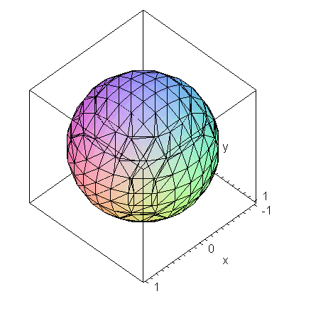
> eq[1] := x^2 + y^2 + z^2 = 1;
 

x^2+y^2+z^2 = 1 

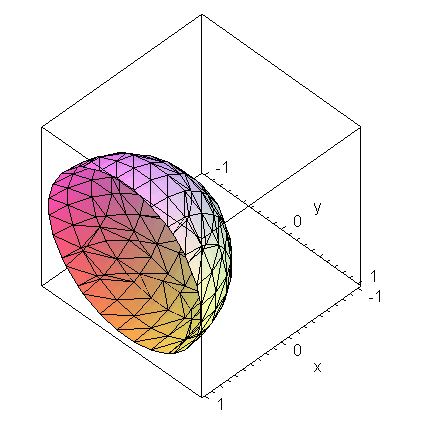
> eq[2] := x^2 + y^2 + z^2 = 2*x;
 

x^2+y^2+z^2 = 2*x 

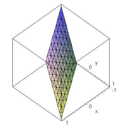
> eq[3] := 2*x - 3*y = z;
 

2*x-3*y = z 


Use plots to see the surfaces represented by these equations in 3-dimensional space. 


> implicitplot3d(eq[1], x=-1..1, y=-1..1, z=-1..1, axes=BOXED);
 

Plot 


> implicitplot3d(eq[2], x=-1..1, y=-1..1, z=-1..1, axes=BOXED);
 

Plot 


> implicitplot3d(eq[3], x=-1..1, y=-1..1, z=-1..1, axes=BOXED);
 

Plot 


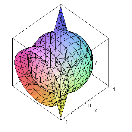
The following command shows all three surfaces in one plot. 

By dragging with the mouse, you can rotate the plot to see different views. 


> implicitplot3d({eq[1],eq[2],eq[3]}, x=-1..1, y=-1..1, z=-1..1, axes=BOXED);
 

Plot 

>


Problem:  Find the points of intersection of the three surfaces represented above. 


Solution:  The solution is readily obtained by applying Groebner basis techniques. 


> F := [seq(lhs(eq[i])-rhs(eq[i]), i = 1..3)];
 

[x^2+y^2+z^2-1, x^2+y^2+z^2-2*x, 2*x-3*y-z] 

> G := Groebner[Basis](F, plex(x,y,z));
 

[40*z^2-8*z-23, 3*y+z-1, 2*x-1] 

> _EnvExplicit := true;
 

true 

> soln := solve(convert(G,'set'), {x,y,z});
 

{z = 1/10+3/20*26^(1/2), x = 1/2, y = 3/10-1/20*26^(1/2)}, {x = 1/2, y = 3/10+1/20*26^(1/2), z = 1/10-3/20*26^(1/2)}
 

> evalf(soln);
 

{y = 0.450490243e-1, z = .8648529271, x = .5000000000}, {x = .5000000000, y = .5549509757, z = -.6648529271}
 

>
 

Concluding Remarks 

The textbook [Geddes92] contains a chapter devoted to algorithms for Groebner bases. For further reading on the solution of systems of polynomial equations and related topics, the textbook [Cox92] is highly recommended. 


Digression: What is a "Closed Form" Solution? 

Chapter Synopsis 

The concept of a "closed form" solution is seen to have varying interpretations, depending on the problem-solving context. 


Example 1:  Polynomial Root Finding 

The following polynomial is cubic in x, so there are three roots. 

> restart;
 

> cubic_poly := x^3 + (a+2)*x^2 + 4*a*(x+1);
 

x^3+(a+2)*x^2+4*a*(x+1) 

> solve(cubic_poly, x);
 

-2, -1/2*a+1/2*(a^2-8*a)^(1/2), -1/2*a-1/2*(a^2-8*a)^(1/2) 

The result is presented in the form of three explicit solutions. 


However, it is sometimes more useful for further computation if we let solutions which are not rational numbers be expressed implicitly in terms of Maple's RootOf notation. 

We can request this mode by setting the following environment variable. 

> _EnvExplicit := false;
 

false 

> solve(cubic_poly, x);
 

-2, RootOf(_Z^2+a*_Z+2*a) 


It is perhaps more readily agreed that the implicit notation is convenient if we consider the case of a quartic polynomial. 


> quartic_poly := x^4 - 1/3*x^3 + 1/2*x^2 + 10*x - 25;
 

x^4-1/3*x^3+1/2*x^2+10*x-25 

> solve(quartic_poly, x);
 

RootOf(6*_Z^4-2*_Z^3+3*_Z^2+60*_Z-150, label = _L1) 

> _EnvExplicit := true;
 

true 

> solve(quartic_poly, x);
 

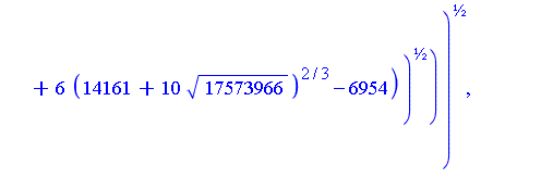
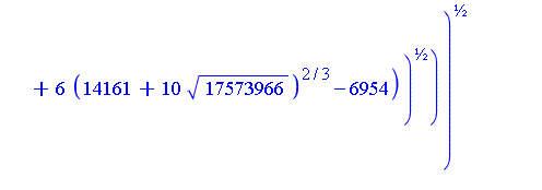
1/12+1/12*((-11*(14161+10*17573966^(1/2))^(1/3)+6*(14161+10*17573966^(1/2))^(2/3)-6954)/(14161+10*17573966^(1/2))^(1/3))^(1/2)+1/12*I*((22*(14161+10*17573966^(1/2))^(1/3)*((-11*(14161+10*17573966^(1/2...


Further manipulation with the complicated expressions appearing in the solution of quartic_poly are often difficult.  In contrast, manipulation with the RootOf notation can be straightforward. 


As one example of the use of implicit notation, consider the following integral. 


> r := Int(1/quartic_poly, x);
 

Int(1/(x^4-1/3*x^3+1/2*x^2+10*x-25), x) 


> value(r);
 

6*(sum(_R*ln(x-814211272993084425/42405712658*_R^3+4988433295703025/42405712658*_R^2-131392052753859/339245701264*_R+440047432655/1017737103792), _R = RootOf(47449708200*_Z^4-649953*_Z^2-4354*_Z-9)))
 

The above result is much more compact than an explicit result, and it is also much easier to evaluate and otherwise to manipulate in further computations. 


Of course, it we try to solve a polynomial of degree 5 which is irreducible over the rationals then the solution cannot be expressed in terms of radicals, hence implicit notation is necessary regardless of the setting of _EnvExplicit . 


> q := x^5 + x^3 + 2*x^2 + 2*x + 1;
 

x^5+x^3+2*x^2+2*x+1 

> solve(q, x);
 

RootOf(_Z^5+_Z^3+2*_Z^2+2*_Z+1, index = 1), RootOf(_Z^5+_Z^3+2*_Z^2+2*_Z+1, index = 2), RootOf(_Z^5+_Z^3+2*_Z^2+2*_Z+1, index = 3), RootOf(_Z^5+_Z^3+2*_Z^2+2*_Z+1, index = 4), RootOf(_Z^5+_Z^3+2*_Z^2+...


Alternatively, the polynomial can be solved in approximate floating-point arithmetic by applying the command.  Here we ask for all the roots in the complex field. 


> fsolve(q, x, complex);
 

-.7344760654, -.4130976855-.6665875516*I, -.4130976855+.6665875516*I, .7803357182-1.266870993*I, .7803357182+1.266870993*I
 

>
 

Example 2:  Solving Non-polynomial Equations 

> restart;
 

> r := solve(x=cos(x), x);
 

RootOf(_Z-cos(_Z)) 


To compute a floating-point approximation for apply the command. 

> evalf(r);
 

.7390851332 


Compare the following two cases. 


> solve(exp(x)=y, x);
 

ln(y) 


Yes, it is well known that the inverse of the exponential function is the natural logarithm function. 


> solve(x*exp(x)=y, x);
 

LambertW(y) 


This function is not so well known (yet).  Until recent years, the latter result would have been expressed in the implicit notation 


> implicit_soln := RootOf(_Z*exp(_Z)-y);
 

RootOf(_Z*exp(_Z)-y) 


and we could manipulate this form;  for example, 


> series(implicit_soln, y);
 

series(y-y^2+3/2*y^3-8/3*y^4+125/24*y^5+O(y^6),y,6) 

which agrees with the series solution of the explicit function known as LambertW: 

> series(LambertW(y), y);
 

series(y-y^2+3/2*y^3-8/3*y^4+125/24*y^5+O(y^6),y,6) 


The function is defined by the above equation;  i.e. it is defined by the property that . 


See the following help page for detailed information. 

> ?LambertW


There are many equations whose roots can be expressed in terms of the LambertW function.  Here is one more example. 


> eqn := ln(cos(2*Pi*x)^2/(y^2+1)) = y*cos(2*Pi*x);
 

ln(cos(2*Pi*x)^2/(y^2+1)) = y*cos(2*Pi*x) 

> soln := solve(eqn, x);
 

1/2*(Pi-arccos(2*LambertW(-1/2*(y^2*(y^2+1))^(1/2))/y))/Pi, 1/2*(Pi-arccos(2*LambertW(1/2*(y^2*(y^2+1))^(1/2))/y))/Pi
 

> plot(soln[1], y=0..1);
 

Warning, unable to evaluate the function to numeric values in the region; see the plotting command's help page to ensure the calling sequence is correct 

Error, empty plot 

> evalf( eval(soln[1], y=1/2) );
 

0.+.1808043812*I 

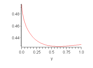
> plot(soln[2], y=0..1);
 

Plot 

> evalf( eval(soln[2], y=1/2) );
 

.4260877916 


Find the point of minimum value of the solution on the interval . 


> deriv := diff(soln[2],y);
 

1/2*((2*y*(y^2+1)+2*y^3)*LambertW(1/2*(y^2*(y^2+1))^(1/2))/(y^3*(y^2+1)*(1+LambertW(1/2*(y^2*(y^2+1))^(1/2))))-2*LambertW(1/2*(y^2*(y^2+1))^(1/2))/y^2)/((1-4*LambertW(1/2*(y^2*(y^2+1))^(1/2))^2/y^2)^(...
 

> fsolve(deriv=0, y, 0..1);
 

.6147342480 

>
 

Example 3: Functions Defined via the RootOf Construct 

Suppose that we wish to solve the equation    where is a parameter in the range . 


> restart;
 

> eqn := cos(2*x) = tan(alpha*x/Pi);
 

cos(2*x) = tan(alpha*x/Pi) 

> soln := solve(eqn, x);
 

1/2*RootOf(_Z*alpha-2*arctan(cos(_Z))*Pi) 


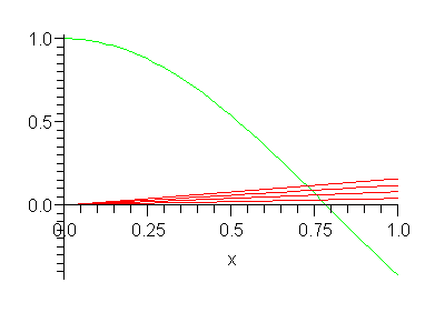
Look at the graphs of and , for some values of , to see where the graphs cross. 


> leqn := lhs(eqn);  reqn := rhs(eqn);
 

cos(2*x) 

tan(alpha*x/Pi) 

> graph[0] := plot( leqn, x=0..1, color=green ):
 

> for k from 1 to 4 do
 graph[k] := plot( eval(reqn,alpha=k/8), x=0..1, color=red )
od:
 

> plots[display]({seq(graph[k],k=0..4)});
 

Plot 


We see that for values of in the range there is a real root (a crossover point) in the interval . 


Define the function which is the solution of this equation. 


> H := unapply(soln, alpha);
 

proc (alpha) options operator, arrow; 1/2*RootOf(_Z*alpha-2*arctan(cos(_Z))*Pi) end proc 

Numerically evaluate for various values of . 


> for k from 1 to 5 do
 'H'(k/10) = evalf(H(k/10))
od;
 

H(1/10) = .7730903215 

H(1/5) = .7611417750 

H(3/10) = .7495192375 

H(2/5) = .7381942900 

H(1/2) = .7271425665 

>
 

Symbolic Manipulation of the RootOf Construct 

The function defined via the construct can be not only evaluated, it can also be manipulated mathematically. 


For example, compute a series expansion. 


> ser_H := series(H(alpha), alpha);
 

series(1/4*Pi-1/8*alpha+1/16/Pi*alpha^2-1/256*(8+Pi^2)/Pi^2*alpha^3+1/128*(2+Pi^2)/Pi^3*alpha^4-1/16384*(128+160*Pi^2+3*Pi^4)/Pi^4*alpha^5+O(alpha^6),alpha,6)


Perhaps we wish to know the rate of change of the solution:   


> diff_H := diff(H(alpha), alpha);
 

-1/2*RootOf(_Z*alpha-2*arctan(cos(_Z))*Pi)/(alpha+2*sin(RootOf(_Z*alpha-2*arctan(cos(_Z))*Pi))*Pi/(1+cos(RootOf(_Z*alpha-2*arctan(cos(_Z))*Pi))^2))


or, for small values of the derivative is well approximated by differentiating the series: 


> diff(ser_H, alpha);
 

series(-1/8+1/8/Pi*alpha-3/256*(8+Pi^2)/Pi^2*alpha^2+1/32*(2+Pi^2)/Pi^3*alpha^3-5/16384*(128+160*Pi^2+3*Pi^4)/Pi^4*alpha^4+O(alpha^5),alpha,5)


Note: We get the same series expansion by directly expanding the expression diff_H : 


> normal( series(diff_H, alpha, 5) );
 

series(-1/8+1/8/Pi*alpha-3/256*(8+Pi^2)/Pi^2*alpha^2+1/32*(2+Pi^2)/Pi^3*alpha^3-5/16384*(128+160*Pi^2+3*Pi^4)/Pi^4*alpha^4+O(alpha^5),alpha,5)


Look at a graph of by plotting the series approximation (first convert the series to a polynomial). 


> poly_H := convert(ser_H, polynom);
 

1/4*Pi-1/8*alpha+1/16*alpha^2/Pi-1/256*(8+Pi^2)*alpha^3/Pi^2+1/128*(2+Pi^2)*alpha^4/Pi^3-1/16384*(128+160*Pi^2+3*Pi^4)*alpha^5/Pi^4
 

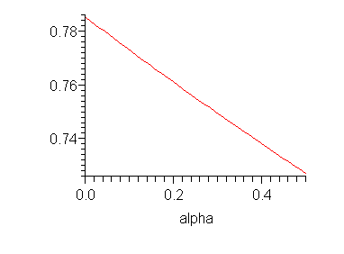
> plot(poly_H, alpha=0..1/2);
 

Plot 

>
 

Final Remarks About the RootOf Construct 

We defined the function    . 


Is the function a closed form solution? 


In the traditional sense, no. 


But in a computer algebra system, when we have given a name (such as ) to a function and, more importantly, when we can perform mathematical manipulations (symbolic as well as numerical) with this function, then is it really a lower class function? 

Is it less useful than a solution expressed in terms of functions which have previously been given names in the mathematical literature, such as arctan, or EllipticK, or a more recent entry into the literature, LambertW ? 


>


Symbolic Integration 

Chapter Synopsis 

The Risch integration algorithm for computing indefinite integrals (antiderivatives) of transcendental elementary functions is described. Extensions of this algorithm to handle algebraic functions, and to the case of non-elementary special functions, are mentioned briefly with pointers to the relevant literature. 


On the problem of computing definite integrals in closed form, some practical issues associated with the application of the Fundamental Theorem of Calculus are described. For some particular classes of definite integrals involving special functions, current research work is briefly described in which the approach is to convert the integrand to a Meijer G function representation, to apply known formulas for definite integrals of products of Meijer G functions, and then to convert the result, if possible, to a representation in terms of standard functions. 


Risch Algorithm for Elementary Functions 

The Problem 

Given a function , determine whether there exists a function such that 


i.e. determine an indefinite integral, or antiderivative, of .  We will write 


where we do not explicitly write the arbitrary constant of integration. 


A detailed development of the Risch integration algorithm presented here can be found in the textbook [Geddes92]. Additional material on the Risch algorithm appears in [Bronstein90b], [Bronstein97]. 


In this presentation, examples will be shown using the Maple computer algebra system.  

Example 1.1 

> restart;
 

> f := x*(x+1)*( (x^2*exp(2*x^2) - ln(x+1)^2)^2 +
2*x*exp(3*x^2)*( x - (2*x^3+2*x^2+x+1)*ln(x+1) )) /
((x+1)*ln(x+1)^2 - (x^3+x^2)*exp(2*x^2) )^2:


> Int(f,x);
 

Int(x*(x+1)*((x^2*exp(2*x^2)-ln(x+1)^2)^2+2*x*exp(3*x^2)*(x-(2*x^3+2*x^2+x+1)*ln(x+1)))/((x+1)*ln(x+1)^2-(x^3+x^2)*exp(2*x^2))^2, x)


> value(%);
 

x-ln(x+1)+exp(x^2)*x*ln(x+1)/(x^2*exp(2*x^2)-ln(x+1)^2)-1/2*ln(-exp(x^2)*x+ln(x+1))+1/2*ln(exp(x^2)*x+ln(x+1))
 

>
 

Defining the function field 

The Risch integration algorithm is a decision procedure by which we mean that given an integrand , the algorithm will determine: 

  • Does there exist a function in a specified class of functions such that ?
 

  • If yes then determine .
 

If the answer to the existence question is no then the algorithm has constructed a proof of nonexistence. 


Such a decision procedure is only possible in a context where we have clearly specified the class of functions (the function field) containing . For example, we will consider the field of elementary functions. In this function field, the Risch algorithm will determine that the integral does not exist. However, if we allow the question to be expanded beyond the field of elementary functions then this integral can be expressed, as shown below by Maple. 


> Int(exp(-x^2), x) = int(exp(-x^2), x);
 

Int(exp(-x^2), x) = 1/2*Pi^(1/2)*erf(x) 

>
 

Definition of Elementary Functions 

Let be a differential field (i.e. a function field on which derivation is defined) and let be a differential extension field of .  Let the derivation operation be denoted by prime ( ' ) . 

  • For in , if there exists in such that  theta^`'` = u^`'`/u  then we write    and  is called logarithmic over .
 

  • For in , if there exists in such that  theta^`'`/theta = u^`'`  then we write    and  is called exponential over .
 

  • For in , if there exists a polynomial in [] such that    then is called algebraic over .


  • in  is transcendental over if is not algebraic over .


  •  is called a transcendental elementary extension of  if    where each is transcendental and either logarithmic or exponential over the field   .
 

  • Similarly, is an elementary extension of if each is logarithmic, exponential or algebraic over .


  • If denotes a differential field of rational functions over a constant field  (a subfield of the complex numbers) and if is an elementary extension of then is called a field of elementary functions.
 

  • Similarly, is called a field of transcendental elementary functions if is a transcendental elementary extension of .


Notation for elementary functions 

Note that the common notation for elementary functions does not make it clear that an elementary function can be described using only the three types of extensions defined above. 


Examples in common notation 

> Int(1/(1+x^2), x) = int(1/(1+x^2), x);
 

Int(1/(1+x^2), x) = arctan(x) 

> Int(cos(x), x) = int(cos(x), x);
 

Int(cos(x), x) = sin(x) 

> Int(1/sqrt(1-x^2), x) = int(1/sqrt(1-x^2), x);
 

Int(1/(1-x^2)^(1/2), x) = arcsin(x) 

> Int(arccosh(x), x) = int(arccosh(x), x);
 

Int(arccosh(x), x) = x*arccosh(x)-(x-1)^(1/2)*(x+1)^(1/2) 

>


In the examples above, each integrand and each integral result involves only elementary functions. To see that these functions conform to the definition of elementary functions of the preceding section, we must convert the functions to complex exp-log form. 


The same examples in exp-log notation 

> Int(1/(1+x^2), x) = convert(int(1/(1+x^2), x), 'expln');
 

Int(1/(1+x^2), x) = 1/2*I*(ln(1-I*x)-ln(1+I*x)) 

> Int(1/2*exp(I*x) + 1/2*exp(-I*x), x) = int(1/2*exp(I*x) + 1/2*exp(-I*x), x);
 

Int(1/2*exp(I*x)+1/2*exp(-I*x), x) = -1/2*I*exp(I*x)+1/2*I*exp(-I*x) 

> Int(1/sqrt(1-x^2), x) = convert(int(1/sqrt(1-x^2), x), 'expln');
 

Int(1/(1-x^2)^(1/2), x) = -I*ln((1-x^2)^(1/2)+I*x) 

> Int(convert(arccosh(x),'expln'), x) = int(convert(arccosh(x),'expln'), x);
 

Int(ln(x+(x-1)^(1/2)*(x+1)^(1/2)), x) = ln(x+(x-1)^(1/2)*(x+1)^(1/2))*x-(x-1)^(1/2)*(x+1)^(1/2)
 

>


We can now see a relationship between the input (the integrand) and the output (the integral result).  Namely, the types of functions which can appear in the integral result are the same functions that appear in the integrand plus, in some cases, new log extensions.  This fact is known as Liouville's Principle: the only new functions needed are constant multiplies of log extensions. 


The common notation hides this relationship. 


Liouville's Principle 

Theorem 1 

Given in an elementary function field , , if it exists as an elementary function, can be expressed in the form 


with   in ,   constants,  and   in . 


Note: The constants may involve new algebraic number extensions. 


Integral of a rational function 

Given a rational function , Liouville's Principle states that its integral can be expressed as a rational function plus (possibly) some constant multiples of functions. (Note that Maple's notation for the natural logarithm function is rather than .) 


For the case of rational functions, the integral always exists as an elementary function. 


Example 1.2 


> Int(1/(x^2+2*x+1), x) = int(1/(x^2+2*x+1), x);
 

Int(1/(x^2+2*x+1), x) = -1/(x+1) 

Remark: No terms required in the above example. 


> Int(1/(x^3+x), x) = int(1/(x^3+x), x);
 

Int(1/(x^3+x), x) = -1/2*ln(1+x^2)+ln(x) 

Remark: No algebraic number extensions required in the above example. 


> Int(1/(x^2-2), x) = `int/risch`(1/(x^2-2), x);
 

Int(1/(x^2-2), x) = 1/4*2^(1/2)*ln(x-2^(1/2))-1/4*2^(1/2)*ln(x+2^(1/2))
 

Remark: In the latter example, the constant field needed to be extended by the algebraic number . 

>


Minimal algebraic extensions are desired for efficiency. 

For example, from above noting that    would lead to the following representation of the integral: 


 . 


Goal:  Avoid introducing algebraic numbers except when necessary. 


Hermite Reductions for the Rational Part 

We want to reduce the problem as follows: 


where    and where    is monic and square-free. 


Hermite's method is a classical method to achieve this reduction. The reduction is accomplished using basic polynomial operations and without introducing any algebraic number extensions.  The method is summarized here. 


Step 1:  Euclidean division with remainder yields 


where    or   . 


Step 2:  Square-free factorization yields 


where  gcd(q[i](x), q[i](x)^`'`) = 1  for all , 

and where    for . 


Step 3:  Partial fraction expansion yields 


where   . 


We now have 

. 


Step 4:  Hermite reductions must be applied for each integrand where the denominator is a power > of a square-free factor. 

After this step, each integral that remains will have a square-free denominator. 

Consider one integral    with > . 

Apply the Extended Euclidean Algorithm to solve:   s(x)*q[i](x)+t(x)*q[i](x)^`'` = r[i, j](x) . 

This yields  Int(r[i, j](x)/q[i](x)^j, x) = Int(s(x)/q[i](x)^(j-1), x)+Int(t(x)*q[i](x)^`'`/q[i](x)^j, x)  . 

Integration by parts yields 

Int(t(x)*q[i](x)^`'`/q[i](x)^j, x) = -t(x)/((j-1)*q[i](x)^(j-1))+Int(t(x)^`'`/((j-1)*q[i](x)^(j-1)), x)
Int(t(x)*q[i](x)^`'`/q[i](x)^j, x) = -t(x)/((j-1)*q[i](x)^(j-1))+Int(t(x)^`'`/((j-1)*q[i](x)^(j-1)), x)  .


Note the contribution to the rational part of the result. 

Hermite reductions can be continued until only square-free denominators remain. 


Example 1.3 

> p := x^6+5*x^5+10*x^4+50*x^3+25*x^2+127*x-1:
 

> q := x^4+10*x^2+25:


The integral we wish to compute is 


> Int(p/q, x);
 

Int((x^6+5*x^5+10*x^4+50*x^3+25*x^2+127*x-1)/(x^4+10*x^2+25), x) 

> r := rem(p, q, x, 'P');
 

-1+2*x 

> P;
 

x^2+5*x 

> int_P := int(P, x);
 

1/3*x^3+5/2*x^2 


Euclidean division with remainder has yielded: 


> Int(p/q, x) = int_P + Int(r/q, x);
 

Int((x^6+5*x^5+10*x^4+50*x^3+25*x^2+127*x-1)/(x^4+10*x^2+25), x) = 1/3*x^3+5/2*x^2+Int((-1+2*x)/(x^4+10*x^2+25), x)


> q_sqrfree := convert(q, sqrfree, x);
 

(x^2+5)^2 

> q2 := x^2 + 5;
 

x^2+5 

In this case, the square-free factorization of the denominator is 

 with    and   . 


The problem has been reduced to 


> Int(p/q, x) = int_P + Int(r/q2^2, x);
 

Int((x^6+5*x^5+10*x^4+50*x^3+25*x^2+127*x-1)/(x^4+10*x^2+25), x) = 1/3*x^3+5/2*x^2+Int((-1+2*x)/(x^2+5)^2, x)


Apply Hermite reduction to the remaining integral which is of the form    with . 


The Extended Euclidean Algorithm is invoked as follows. 


> gcdex(q2, diff(q2,x), r, x, 's', 't');
 

> s;
 

-1/5 

> t;
 

1+1/10*x 

> j := 2:


The Hermite reduction formula takes the form 


> Int(r/q2^j, x) = -t/((j-1)*q2^(j-1)) + Int((s+diff(t,x)/(j-1))/q2^(j-1), x);
 

Int((-1+2*x)/(x^2+5)^2, x) = -(1+1/10*x)/(x^2+5)+Int(-1/10/(x^2+5), x)


and therefore the original integral has been reduced to 


> Int(p/q, x) = int_P + rhs(%);
 

Int((x^6+5*x^5+10*x^4+50*x^3+25*x^2+127*x-1)/(x^4+10*x^2+25), x) = 1/3*x^3+5/2*x^2-(1+1/10*x)/(x^2+5)+Int(-1/10/(x^2+5), x)
 

>
 

Rothstein-Trager Theorem for the Logarithmic Part 

The problem is to express    where    and    is square-free. 

Classical approach:  Factor B(x) over its splitting field, and then a partial fraction expansion determines the terms. 

But such a factorization may be much more expensive than necessary. 


Theorem 2  (Rothstein-Trager Theorem) 


where are the distinct roots of  R(z) = resultant(A(x)-z*B(x)^`'`, B(x), x) 

and where are the polynomials  v[i](x) = gcd(A(x)-c[i]*B(x)^`'`, B(x)) . 

Moreover, this expresses the integral using the minimal algebraic extension field. 


Remark: The roots of may introduce new algebraic numbers. 


Example 1.4 


From Example 1.3 the remaining integral is 


> A := -1/10:  B := x^2 + 5:
 

> Int(A/B, x);
 

Int(-1/10/(x^2+5), x) 

> R := resultant(A - z*diff(B,x), B, x);
 

20*z^2+1/100 

> (c1,c2) := solve(R=0, z);
 

1/100*I*5^(1/2), -1/100*I*5^(1/2) 

> v1 := gcd(A - c1*diff(B,x), B);
 

-I*5^(1/2)+x 

> v2 := gcd(A - c2*diff(B,x), B);
 

I*5^(1/2)+x 


Therefore the integral can be expressed as follows. 


> Int(A/B, x) = c1*log(v1) + c2*log(v2);
 

Int(-1/10/(x^2+5), x) = 1/100*I*5^(1/2)*ln(-I*5^(1/2)+x)-1/100*I*5^(1/2)*ln(I*5^(1/2)+x)
 

>
 

In this case, the result is identical to that obtained by the "classical approach" where the denominator is completely factored. 


Example 1.5 


One of the integrals from Example 1.2 is 


> A := 1:  B := x^3+x:
 

> Int(A/B, x);
 

Int(1/(x^3+x), x) 

> R := resultant(A - z*diff(B,x), B, x);
 

(1-z)*(2*z+1)^2 

> solve(R=0, z);
 

1, -1/2, -1/2 

The distinct roots are 

> (c1,c2) := (1,-1/2);
 

1, -1/2 

> v1 := gcd(A - c1*diff(B,x), B);
 

x 

> v2 := gcd(A - c2*diff(B,x), B);
 

1+x^2 


Therefore the integral can be expressed as follows. 


> Int(A/B, x) = c1*log(v1) + c2*log(v2);
 

Int(1/(x^3+x), x) = ln(x)-1/2*ln(1+x^2) 


In contrast, the "classical" approach would require a complete factorization of the denominator 


> factored_B := factor(B,I);
 

x*(x+I)*(x-I) 

> integrand := convert(A/factored_B, parfrac, x);
 

1/x-1/2/(x+I)-1/2/(x-I) 

from which we see that the integral is 


> Int(A/B, x) = map(`int/risch`, integrand, x);
 

Int(1/(x^3+x), x) = ln(x)-1/2*ln(x+I)-1/2*ln(x-I) 

>
 

The Rothstein-Trager method avoids introducing the algebraic number extension    in this example. 

Computational cost increases significantly with each new algebraic number extension, so it is important to use the minimal number of extensions required by the problem. 


The case of transcendental elementary functions 


Step 1: Determine a description    of a function field containing the integrand . 

 is the constant field (we dynamically extend it to include any algebraic numbers which may arise). 

We must ensure that each is a new transcendental extension.  (This allows the manipulation of the integrand as a rational expression in the independent symbols .) 


Example 1.6 

For the integral 

> Int(1/ln(x), x);
 

Int(1/ln(x), x) 

the integrand lies in the function field where is a logarithmic extension of the rational function field . 

In this field the integrand is 

> 1/theta;
 

1/theta 

>
 

Example 1.7 

For the integral 

> Int((x^3+2*x)*cos(x^2)+x*sin(x^2), x);
 

Int((x^3+2*x)*cos(x^2)+x*sin(x^2), x) 

by converting the integrand to complex - form, the problem can be expressed in the form 


> Int((x^3+2*x)*(exp(I*x^2)+exp(-I*x^2))/2 - 1/2*I*x*(exp(I*x^2)-exp(-I*x^2)), x);
 

Int(1/2*(x^3+2*x)*(exp(I*x^2)+exp(-I*x^2))-1/2*I*x*(exp(I*x^2)-exp(-I*x^2)), x)
 

and we can view the integrand as an element of the function field    where .  (Note: .) 

In this field the integrand is 

> 1/2*(x^3+2*x)*(theta + 1/theta) - 1/2*I*x*(theta - 1/theta);
 

1/2*(x^3+2*x)*(theta+1/theta)-1/2*I*x*(theta-1/theta) 

>
 

Example 1.8 


For the integral presented in Example 1.1 

> Int(x*(x+1)*( (x^2*exp(2*x^2) - ln(x+1)^2)^2 +
2*x*exp(3*x^2)*( x - (2*x^3+2*x^2+x+1)*ln(x+1) )) /
((x+1)*ln(x+1)^2 - (x^3+x^2)*exp(2*x^2) )^2, x);
 

Int(x*(x+1)*((x^2*exp(2*x^2)-ln(x+1)^2)^2+2*x*exp(3*x^2)*(x-(2*x^3+2*x^2+x+1)*ln(x+1)))/((x+1)*ln(x+1)^2-(x^3+x^2)*exp(2*x^2))^2, x)
 

we can view the integrand as an element of the function field    where and . 

Note that the two exponential terms    and    cannot be considered as independent extensions because there is an algebraic relationship between them. Rather, we choose to represent these terms in the form    and    which involves a single transcendental extension   . 

>


Step 2: Consider the integrand as a rational expression in the field : 


where denotes the last extension and where   .  In other words, and are viewed as polynomials in the domain [] .  Normalize such that and is monic. 


The algorithm proceeds in a manner similar to rational function integration; specifically, Hermite reductions followed by the application of a Rothstein-Trager Theorem.  In particular, the algorithm will apply polynomial operations.  We consider separately the cases where the last extension    is a logarithmic extension or an exponential extension. 


Integral of a logarithmic extension 

Suppose that the last extension    is a logarithmic extension, i.e.  theta^`'` = u^`'`/u  for some function in .  Applying Euclidean division with remainder yields   . 

We now have two integrals to consider:  (1) the integral of the polynomial part;  and (2) the integral of the rational part.  This time (unlike the case of rational function integration) the integral of the polynomial part is nontrivial; indeed, task (1) is the harder of the two parts.  We first consider task (2). 


Hermite Reductions for the Rational Part (log extension) 

This case mimics the Hermite method for rational functions.  Applying square-free factorization of the denominator yields    where this means "square-free as a polynomial in ."  For application in subsequent steps of the algorithm, we need to know that the following theorem holds. 


Theorem 3:  If is a monic polynomial which is square-free as a polynomial in the symbol and if    for some function then 

                   gcd(v(theta), v(theta)^`'`) = 1 

where the latter differentiation is with respect to . 


Then applying partial fraction expansion, we get 

   where     . 


For each integral with a denominator containing a power   > , apply the Extended Euclidean Algorithm to solve 

                    s(theta)*b[i](theta)+t(theta)*b[i](theta)^`'` = r[i, j](theta) . 

As in rational function integration, apply integration by parts to obtain the Hermite reduction: 

Int(r[i, j](theta)/b[i](theta)^j, x) = -t(theta)/((j-1)*b[i](theta)^(j-1))+Int((s(theta)+t(theta)^`'`/(j-1))/b[i](theta)^(j-1), x)
Int(r[i, j](theta)/b[i](theta)^j, x) = -t(theta)/((j-1)*b[i](theta)^(j-1))+Int((s(theta)+t(theta)^`'`/(j-1))/b[i](theta)^(j-1), x) .
 

Continuing such reductions until no remaining integral has a denominator containing a power   > , we reduce the integration problem to one in which the denominator is square-free. 


Rothstein-Trager Theorem: log extension 

The problem is to express    where   ,    is square-free, and where    is a logarithmic extension. 


Theorem 4  (Rothstein-Trager Theorem: log extension) 

(i)    is elementary if and only if all of the roots of 

         R(z) = resultant(A(theta)-z*B(theta)^`'`, B(theta), theta) 


are constants.  In other words, the primitive part of with respect to the variable must have constant coefficients. 


(ii)  If    is elementary then 


where are the distinct roots of and where are defined by 

         v[i](theta) = gcd(A(theta)-c[i]*B(theta)^`'`, B(theta)) . 


Moreover, this expresses the integral using the minimal algebraic extension field. 


Example 1.9 

Consider the following integral. 

> restart;
 

> Int(1/ln(x), x);
 

Int(1/ln(x), x) 

The integrand is    in the function field where . 

A resultant computation (Rothstein-Trager Theorem) is applicable. 


> A := 1:  B := theta:
 

> diff_B := diff(ln(x), x);
 

1/x 

> R := resultant(A - z*diff_B, B, theta);
 

(x-z)/x 

The single root of is which is not a constant. 

Therefore the original integral is not elementary. 

>
 

Example 1.10 

The integral 

> restart;
 

> Int(1/(x*ln(x)), x);
 

Int(1/(x*ln(x)), x) 

has integrand    in the function field where . 

This time, the resultant computation is as follows. 

> A := 1:  B := x*theta:
 

> diff_B := subs(ln(x)=theta, diff(subs(theta=ln(x), B), x));
 

theta+1 

> R := resultant(A - z*diff_B, B, theta);
 

x*(-1+z) 

The single root of is and the integral is elementary.  Specifically, 

> c[1] := 1;  v[1] := gcd(A - c[1]*diff_B, B);
 

1 

theta 

and the integral is 

> c[1]*ln(v[1]);
 

ln(theta) 

In other words, 

> Int(1/(x*ln(x)), x)  =
subs(theta=ln(x), c[1]*ln(v[1]));
 

Int(1/(x*ln(x)), x) = ln(ln(x)) 

>
 

Polynomial Part (log extension) 

For the integration of the "polynomial part", the integrand is a polynomial in the log extension : 


with    in    and we can conclude that 


.
 

Note that the last term indicates that some new log extensions may arise. 


Differentiating and equating coefficients of powers of the transcendental symbol , we get: 

         0 = B[k+1]^`'` 

         A[k] = (k+1)*B[k+1]*theta^`'`+B[k]^`'` 

         A[k-1] = k*B[k]*theta^`'`+B[k-1]^`'` 

                 . . . 

                 . . . 

         A[1] = 2*B[2]*theta^`'`+B[1]^`'` 

         A[0] = B[1]*theta^`'`+(B[0]^`*`)^`'` 

where   . 

We can solve these equations successively, from the top down.  At each step there is an integration operation which requires a recursive invocation of the Risch algorithm.  This works because the integrand lies in the field    involving one less extension.  At any step, if the integral to be computed is not elementary then the algorithm halts with the conclusion that the original integral is not elementary.  Moreover, at any step except the last step, if the result of the recursive integration introduces one or more new log extensions then the algorithm halts with the conclusion that the original integral is not elementary.  At the last step, new log extensions may appear. 


Example 1.11 

The integral 


has integrand    in the field    where   .  If the integral is elementary then 


where the equations to be satisfied are 

         0 = B[2]^`'` 

         1 = 2*B[2]*theta^`'`+B[1]^`'` 

         0 = B[1]*theta^`'`+(B[0]^`*`)^`'`   . 


From the first equation we conclude that   , an arbitrary constant of integration.  Plugging this into the second equation and integrating both sides yields 


or 


where is an arbitrary constant of integration. Equating coefficients of on both sides of the equation, we conclude that and . 

The last equation now becomes 

         0 = (x+b[1])*theta^`'`+(B[0]^`*`)^`'` 

or rearranging (we always leave the term  i*b[i]*theta^`'`  on the right hand side since integration of this term is trivial): 

         -x*theta^`'` = b[1]*theta^`'`+(B[0]^`*`)^`'`   . 

At this point we use the fact that    (i.e. theta^`'` = 1/x )  on the left hand side, and integrate both sides to get 


from which we conclude (by equating coefficients of on both sides of the equation) that and , ignoring the arbitrary constant of integration in this final step. Putting it all together we have 

> theta := ln(x):
 

> B[2] := 0:  B[1] := x:  B[0] := -x:
 

> Int(theta, x) = B[2]*theta^2 + B[1]*theta + B[0];
 

Int(ln(x), x) = x*ln(x)-x 

>
 

Example 1.12 

The integral 


has integrand    in the field    where and .  If the integral is elementary then 


where the equations to be satisfied are 

         0 = B[2]^`'` 

         1 = 2*B[2]*theta[2]^`'`+B[1]^`'` 

         0 = B[1]*theta[2]^`'`+(B[0]^`*`)^`'`   . 


From the first equation we conclude that   , an arbitrary constant of integration.  Plugging this into the second equation and integrating both sides yields 


or 


where is an arbitrary constant of integration. Equating coefficients of on both sides of the equation, we conclude that and . The last equation now becomes 

         0 = (x+b[1])*theta[2]^`'`+(B[0]^`*`)^`'` 

or rearranging: 

         -x*theta[2]^`'` = b[1]*theta[2]^`'`+(B[0]^`*`)^`'`   . 

Since  theta[2]^`'` = theta[1]^`'`/theta[1] ,  i.e. theta[2]^`'` = 1/(x*ln(x)) , substituting for theta[2]^`'` on the left hand side and integrating yields 

            . 

From Example 1.9 we know that the integral appearing here is not elementary. Hence we conclude that    is not elementary. 


Integral of an exponential extension 

Suppose that the last extension    is an exponential extension, i.e.  theta^`'`/theta = u^`'`  for some function in .  Applying Euclidean division with remainder yields   . 

Unlike the logarithmic case, we must remove any power of    from the denominator on the right hand side, and incorporate it into the new "polynomial part":   .  (This can be done.) 

We now have two integrals to consider:  (1) the integral of the polynomial part;  and (2) the integral of the rational part.  Again, task (1) is the harder of the two parts.  We first consider task (2). 


Hermite Reductions for the Rational Part (exp extension) 

This case is very similar to the logarithmic case.  Applying square-free factorization of the denominator yields    where this means "square-free as a polynomial in ."  For application in subsequent steps of the algorithm, we need to know that the following theorem holds. 


Theorem 5:  If is a monic polynomial which is square-free as a polynomial in the symbol and if    for some function then 

                   gcd(v(theta), v(theta)^`'`) = 1 

where the latter differentiation is with respect to , provided that    does not divide . 


Then, exactly as in the logarithmic case, applying partial fraction expansion we get 

   where     . 


For each integral with a denominator containing a power   > , apply the Extended Euclidean Algorithm to solve 

                    s(theta)*b[i](theta)+t(theta)*b[i](theta)^`'` = r[i, j](theta) . 

As before, apply integration by parts to obtain the Hermite reduction: 

Int(r[i, j](theta)/b[i](theta)^j, x) = -t(theta)/((j-1)*b[i](theta)^(j-1))+Int((s(theta)+t(theta)^`'`/(j-1))/b[i](theta)^(j-1), x)
Int(r[i, j](theta)/b[i](theta)^j, x) = -t(theta)/((j-1)*b[i](theta)^(j-1))+Int((s(theta)+t(theta)^`'`/(j-1))/b[i](theta)^(j-1), x) .
 

Continuing such reductions until no remaining integral has a denominator containing a power   > , we reduce the integration problem to one in which the denominator is square-free. 


Rothstein-Trager Theorem: exp extension 

The problem is to express    where   ,    is square-free, and where    is an exponential extension. 


Theorem 6  (Rothstein-Trager Theorem: exp extension) 

(i)    is elementary if and only if all of the roots of 

         R(z) = resultant(A(theta)-z*B(theta)^`'`, B(theta), theta) 


are constants.  In other words, the primitive part of with respect to the variable must have constant coefficients. 


(ii)  If    is elementary then 


where are the distinct roots of ,   are defined by 

         v[i](theta) = gcd(A(theta)-c[i]*B(theta)^`'`, B(theta)) 

and where   . 


Moreover, this expresses the integral using the minimal algebraic extension field. 


Example 1.13 

Consider the following integral. 

> restart;
 

> f := (x*exp(2*x^2)+8*sqrt(2)*x*(exp(x^2)+1)+2*x)/
    (exp(3*x^2)+exp(2*x^2)+2*exp(x^2)+2):
 

> Int(f,x);
 

Int((x*exp(2*x^2)+8*2^(1/2)*x*(exp(x^2)+1)+2*x)/(exp(3*x^2)+exp(2*x^2)+2*exp(x^2)+2), x) 

The integrand is    in the function field where . 


A resultant computation (Rothstein-Trager Theorem) is applicable. 

Keep in mind that    where   . 

> u := x^2:
 

> A := x*theta^2 + 8*sqrt(2)*x*(theta+1) + 2*x:
 

> B := theta^3 + theta^2 + 2*theta + 2:
 

> diff_B := subs(exp(u)=theta, diff(subs(theta=exp(u), B), x));
 

6*theta^3*x+4*x*theta^2+4*x*theta 

> R := resultant(A - z*diff_B, B, theta);
 

-576*x^3*(2+4*z+2*2^(1/2)*z+4*2^(1/2)*z^2+z^2+2*z^3)
 

> solve(R=0, z);
 

-1/2, -2^(1/2), -2^(1/2) 

The distinct roots of are    and    and the integral is elementary.  Specifically, 

> c[1] := -1/2:  c[2] := -sqrt(2):
 

> v[1] := gcd(A - c[1]*diff_B, B);
 

theta+1 

> v[2] := gcd(A - c[2]*diff_B, B);
 

theta^2+2 

The function appearing in Theorem 6 is 

> g := add(-c[i]*degree(v[i],theta), i=1..2) * u;
 

(1/2+2*2^(1/2))*x^2 

and the desired integral is 

> result := g + add(c[i]*ln(v[i]), i=1..2);
 

(1/2+2*2^(1/2))*x^2-1/2*ln(theta+1)-2^(1/2)*ln(theta^2+2)
 

In other words, 

> Int(f,x) = subs(theta=exp(u), result);
 

Int((x*exp(2*x^2)+8*2^(1/2)*x*(exp(x^2)+1)+2*x)/(exp(3*x^2)+exp(2*x^2)+2*exp(x^2)+2), x) = (1/2+2*2^(1/2))*x^2-1/2*ln(exp(x^2)+1)-2^(1/2)*ln((exp(x^2))^2+2)
 

>
 

Polynomial Part (exp extension) 

For the integration of the "polynomial part", the integrand is of the form    with    in   , where    is an exponential extension.  We can conclude that 

. 


Note that the latter summation indicates that some new log extensions may arise. 


Differentiating and equating coefficients of powers of the transcendental symbol , we get: 

         A[j] = B[j]^`'`+j*u^`'`*B[j]  ,   for  

         A[0] = (B[0]^`*`)^`'` 

where   . 

Solving the latter equation for    requires a recursive integration:    where the integrand lies in the field   .  For the general case,   , the equation to be solved for    is known as a Risch differential equation.  This may sound like a backwards step to have reduced an integration problem to the solution of a differential equation!  However, the problem can be solved because we must look for a solution in the field    only.  Nonetheless, this is a difficult problem, in general, for which a complete solution was presented in [Bronstein90a].  See also [Bronstein97]. 


Example 1.14 

The integral 

> Int(exp(-x^2), x);
 

Int(exp(-x^2), x) 

has integrand    in the function field where . 

The solution must take the form    where in is a solution of the Risch differential equation  B[1]^`'`-2*x*B[1] = 1 . 

Since must be a rational function in , one first argues that it must be a polynomial in . This follows because if   had a nontrivial denominator then B[1]^`'`  would have a higher-degree denominator and these denominators could not cancel out to correspond to the right hand side of the differential equation which is the constant 1 .  So assume that    is a nonzero polynomial in with    where   .  But then taking the degree of each side of the differential equation, we get    which is a contradiction.  Hence the given Risch differential equation has no solution in the field    from which we conclude that the original integral is not elementary. 

>
 

Comments on algebraic and mixed extensions 

In the algorithm presented above we considered only transcendental elementary functions. The Risch algorithm for elementary functions also deals with algebraic extensions. For example, if the integral to be computed is    then the integrand lies in the elementary function field    where    is an algebraic extension of and    is a transcendental extension of . The Risch algorithm proceeds generally in the same manner as discussed above except that there are some different technical details (some of them involving concepts from advanced algebra) for algebraic extensions in the most general case. Some references which discuss the integration of elementary functions for the case of algebraic extensions, and mixed transcendental and algebraic extensions, are [Trager84] and [Bronstein90b]. 


Comments on non-elementary extensions 

The power of the Risch algorithm to determine conclusively whether or not a given elementary function has an elementary antiderivative is impressive, in principle. However in most practical problems where the operation of integration arises, it is quite unsatisfactory to receive as a result: "the integral cannot be expressed in elementary terms". For example, the Risch algorithm proves that    cannot be expressed as an elementary function (see Example 1.14) but in a larger function field the integral can be expressed: 

> Int(exp(-x^2), x) = int(exp(-x^2), x);
 

Int(exp(-x^2), x) = 1/2*Pi^(1/2)*erf(x) 

where a special function, the error function, arises. Another case is the following integral which in Example 1.12 was proved to be non-elementary: 

> Int(ln(ln(x)), x) = int(ln(ln(x)), x);
 

Int(ln(ln(x)), x) = ln(ln(x))*x+Ei(1, -ln(x)) 

where another special function, the exponential integral, arises. 

>


It would be ideal if we could extend the elementary function field by an arbitrary number of special functions, as new transcendental extensions, and have a corresponding extended Risch algorithm as a decision procedure for the extended field. At the present time, decision procedures have not been developed for integration in function fields containing many of the commonly-used special functions. However, decision procedures have been developed for some special functions. Early work in this regard is reported in [Cherry85], [Cherry86] where decision procedures are developed for the error function and the logarithmic integral. Additional examples of integrals which can be computed in this context are the following two integrals. 


See [Bronstein97] for a presentation of the state-of-the-art of integration algorithms for transcendental functions. 

Symbolic Solution of Definite Integrals 

Fundamental Theorem of Calculus: practical issues 

We turn now to the problem of computing a definite integral in closed form.  The first concept is that if we are able to express the indefinite integral (antiderivative) then the Fundamental Theorem of Calculus can be applied (under appropriate conditions) to compute the value of the definite integral. In it simplest form, if has antiderivative then   . 

The first problem we encounter with this formula for the value of the definite integral is that it may not be possible to evaluate directly or , but rather it is the limit (an appropriate one-sided limit) which must be computed at each endpoint. Specifically, the formula becomes (suppose that ) : 

 . 


Example 2.1 

> restart;
 

> f := ln(x):
 

We wish to compute the definite integral 

> Int(f, x=0..2);
 

Int(ln(x), x = 0 .. 2) 

We can compute the antiderivative 

> F := int(f, x);
 

x*ln(x)-x 

but direct evaluation of the antiderivative at encounters a logarithmic singularity. However, by taking limits we can compute the result as follows. 

> limit(F, x=2, left) - limit(F, x=0, right);
 

2*ln(2)-2 

Of course, the integration procedure in Maple will do this computation automatically. 

> int(f, x=0..2);
 

2*ln(2)-2 

>


We see that the computation of definite integrals requires the ability to compute limits. In general, computing limits is a nontrivial task. Fortunately, very powerful algorithms are now known for computing limits based on the expansion of functions in generalized series. Once we have expressed a function in a generalized series expansion then the limit can be determined from the leading term of the expansion. 


Example 2.2 

> g := sin(x)/x;
 

sin(x)/x 

> series(g, x=0);
 

series(1-1/6*x^2+1/120*x^4+O(x^5),x,5) 

From the series expansion it is clear what is the limit at . 

> Limit(g, x=0) = limit(g, x=0);
 

Limit(sin(x)/x, x = 0) = 1 


Another example: 


> g := x^x;
 

x^x 

> series(g, x=0, 3);
 

series(1+ln(x)*x+1/2*ln(x)^2*x^2+O(x^3),x,3) 

> Limit(g, x=0) = limit(g, x=0);
 

Limit(x^x, x = 0) = 1 


And another example: 


> g := ln(1-cos(x^2))/(ln(x)*arctan(sqrt(1-x^2)));
 

ln(1-cos(x^2))/(ln(x)*arctan((1-x^2)^(1/2))) 

> series(g, x=0, 4);
 

series(4*(-ln(2)+4*ln(x))/(ln(x)*Pi)-4*(ln(2)-4*ln(x))/(ln(x)*Pi^2)*x^2+O(x^4),x,4)
 

> Limit(g, x=0) = limit(g, x=0);
 

Limit(ln(1-cos(x^2))/(ln(x)*arctan((1-x^2)^(1/2))), x = 0) = 16/Pi 

>


The computation of generalized series expansions, and the computation of limits, requires very sophisticated techniques in the most general case. Some work on this problem was reported in [GeddesGonnet89]. More recent work which develops the theoretical foundation and presents practical algorithms can be found in [Salvy91], [Salvy92], [Richardson96]. 


A difficult  problem which arises in the computation of definite integrals is that the Fundamental Theorem of Calculus can be applied in the manner discussed above only if the integrand and its antiderivative are continuous on the interval . Since the form of antiderivative computed by the Risch integration algorithm can contain logarithmic functions, without special care the condition of continuity may be violated as discussed in [Bronstein97]. See also [Jeffrey93], [Jeffrey97] on the problem of computing continuous antiderivatives. 


Example 2.3 

The following example is discussed in [Bronstein97]. Suppose that the integral to be computed is 

> f := (x^4-3*x^2+6)/(x^6-5*x^4+5*x^2+4):
 

> Int(f, x=1..2);
 

Int((x^4-3*x^2+6)/(x^6-5*x^4+5*x^2+4), x = 1 .. 2) 

It can be verified that the integrand is continuous and positive on the real line, and hence the value of the definite integral must be a positive real number. Applying the integration algorithm in the form discussed in this presentation, the indefinite integral gets expressed in the following form. 

> F := I/2*ln(x^3+I*x^2-3*x-2*I) - I/2*ln(x^3-I*x^2-3*x+2*I);
 

1/2*I*ln(x^3+I*x^2-3*x-2*I)-1/2*I*ln(x^3-I*x^2-3*x+2*I)
 

That is, 

> Int(f, x) = F;
 

Int((x^4-3*x^2+6)/(x^6-5*x^4+5*x^2+4), x) = 1/2*I*ln(x^3+I*x^2-3*x-2*I)-1/2*I*ln(x^3-I*x^2-3*x+2*I)
 

It can easily be verified that the derivative of    is the integrand    and therefore this is a correct formal antiderivative. However, the differential algebra point of view used in developing the integration algorithm takes no account of the analytic concept of branch cuts of logarithmic functions. In this particular example, if we blindly apply the Fundamental Theorem of Calculus we get the following incorrect result for the definite integral. 

> Int(f, x=1..2) = limit(F, x=2, left) - limit(F, x=1, right);
 

Int((x^4-3*x^2+6)/(x^6-5*x^4+5*x^2+4), x = 1 .. 2) = -5/4*Pi+arctan(1/2) 

> evalf(rhs(%));
 

-3.463343209 

This has yielded a value for the integral which is real, but negative, whereas we know that the correct answer must be positive. The presentation in [Bronstein97] shows how to ensure that the integration algorithm computes a continuous antiderivative for this type of problem. In this case, a continuous antiderivative is 

> F_continuous := arctan((x^5 - 3*x^3 + x)/2) + arctan(x^3) + arctan(x);
 

arctan(1/2*x^5-3/2*x^3+1/2*x)+arctan(x^3)+arctan(x)
 

By differentiating, we see that this is a correct antiderivative of the original integrand . 

> simplify( diff(F_continuous, x) );
 

(x^4-3*x^2+6)/(x^6-5*x^4+5*x^2+4) 


This time, direct application of the Fundamental Theorem of Calculus is valid and we obtain the following result for the definite integral. 


> Int(f, x=1..2) = limit(F_continuous, x=2, left) - limit(F_continuous, x=1, right);
 

Int((x^4-3*x^2+6)/(x^6-5*x^4+5*x^2+4), x = 1 .. 2) = arctan(5)+arctan(8)+arctan(2)+arctan(1/2)-1/2*Pi
 

> evalf(rhs(%));
 

2.819842099 

>


A general technique which can be applied when the antiderivative is not guaranteed to be continuous is to find the points of discontinuity of the antiderivative and then to express the integral separately on each subinterval where it is continuous. By computing the appropriate one-sided limits on each subinterval, the correct definite integral is obtained. 


Example 2.4 

In Example 2.3 we had the following discontinuous antiderivative. 

> Int(f, x) = F;
 

Int((x^4-3*x^2+6)/(x^6-5*x^4+5*x^2+4), x) = 1/2*I*ln(x^3+I*x^2-3*x-2*I)-1/2*I*ln(x^3-I*x^2-3*x+2*I)
 

In Maple, the following command will determine the points of discontinuity over the whole real line. 

> discont(F, x);
 

{RootOf(_Z^2-2, -1.414213562), RootOf(_Z^2-2, 1.414213562)}
 

> allvalues(%);
 

{2^(1/2), -2^(1/2)} 


The above notation is expressing the fact that there are two points of discontinuity which are the two roots of a quadratic polynomial. Since we are interested in the definite integral over the interval there is just one relevant point of discontinuity: 

> c := sqrt(2);
 

2^(1/2) 

and the endpoints of integration are 

> a := 1;  b := 2;
 

1 

2 


The correct value of the definite integral on can therefore be computed by using the fact that 


and noting that the antiderivative    is continuous on each of the two subintervals. 

This leads to the following limit computations for the definite integral. 


> Int(f, x=a..b) = limit(F, x=c, left) - limit(F, x=a, right) +
                limit(F, x=b, left) - limit(F, x=c, right);
 

Int((x^4-3*x^2+6)/(x^6-5*x^4+5*x^2+4), x = 1 .. 2) = 3/4*Pi+arctan(1/2) 

> evalf(rhs(%));
 

2.819842099 

>
 

Methods for Special Functions: Generalized hypergeometric function and Meijer G function 

Many non-elementary functions appear in the literature of the mathematical sciences, with names such as Bessel functions, Legendre functions, exponential integrals, elliptic integrals, et cetera. The list of such special functions is quite long. For classes of functions where we have no Risch-like algorithm to compute the indefinite integral, how can we compute integrals that involve such functions which arise in practical problems (assuming that we wish to obtain a closed-form symbolic result if possible)? 


Various special formulas can be programmed into a computer algebra system for integrals which appear in the literature. A particular approach discussed in [Geddes90] derives classes of integral formulas by applying differentiation to the integral definition of various special functions. A more general technique which is capable of obtaining results for a large number of integrals, most often definite integrals on the interval , is to convert the integrand into one of the higher functions: the generalized hypergeometric function or the Meijer G function. We do not have space here to go into details about these functions or about this approach to computing integrals, but we show some examples to illustrate the concept. 


The generalized hypergeometric function and the Meijer G function are discussed in [PBM90]. The same series of books presents a large number of integral formulas involving special functions which computer algebra systems should know how to compute. At the present time, computer algebra systems cannot compute many of the integrals found in these books. 


The general approach being illustrated here to compute a special class of integrals is as follows. 

  • Convert the integrand to a representation in terms of Meijer G functions.
 

  • Apply a formula to express the integral in terms of higher functions.
 

  • Convert the result from a representation in terms of higher functions to a representation in terms of more standard functions (if possible).
 

Note that for definite integrals on  where the integrand involves a product of Meijer G functions, various formulas are available to express the integral. For the problem of converting from a representation in terms of higher functions to a representation in terms of more standard functions (elementary functions and special functions), see [Roach96], [Roach97]. 


Example 2.5 

> restart;
 

> f1 := x^(s-1)*exp(-p*x^4)*erfi(c*x)*erf(c*x):
 

> Int(f1, x=0..infinity);
 

Int(x^(s-1)*exp(-p*x^4)*erfi(c*x)*erf(c*x), x = 0 .. infinity) 

> result1 := value(%) assuming c>0;
 

c^2*p^(-1/2-1/4*s)*hypergeom([1/2, 1, 1/2+1/4*s], [3/4, 5/4, 3/2], 1/4*c^4/p)*GAMMA(1/2+1/4*s)/Pi


The method used was first to convert the integrand into form. 


> f1new := convert(f1, MeijerG, x);
 

-I*x^(s-1)*exp(-p*x^4)*MeijerG([[1], []], [[1/2], [0]], -c^2*x^2)*MeijerG([[1], []], [[1/2], [0]], c^2*x^2)/Pi


Now when we apply the command, it uses a known formula to express such a definite integral involving the product of two functions. 


> int(f1new, x=0..infinity) assuming c>0;
 

c^2*p^(-1/2-1/4*s)*hypergeom([1/2, 1, 1/2+1/4*s], [3/4, 5/4, 3/2], 1/4*c^4/p)*GAMMA(1/2+1/4*s)/Pi
 

which is equal to . 

Of course, for particular values of the parameters we may compute a numerical value. 


> eval(result1, {s=4, p=1, c=1});
 

1/2*hypergeom([1/2, 1], [3/4, 5/4], 1/4)/Pi^(1/2) 

> evalf(%);
 

.3235544850 

>
 

Example 2.6 

> f2 := x^v/(x^2+z^2)*BesselK(v,b*x):
 

> Int(f2, x=0..infinity);
 

Int(x^v*BesselK(v, b*x)/(x^2+z^2), x = 0 .. infinity) 

> value(%) assuming z::real, b>0;
 

1/4*b^(-v)*(b/(1/z^2)^(1/2))^v*Pi^2*(StruveH(-v, b/(1/z^2)^(1/2))-BesselY(-v, b/(1/z^2)^(1/2)))*sec(Pi*v)/(z^2*(1/z^2)^(1/2))


Note that the result of converting the integrand into form is as follows. 


> f2new := convert(f2, MeijerG, x);
 

1/2*x^v*MeijerG([[], []], [[1/2*v, -1/2*v], []], 1/4*b^2*x^2)/(x^2+z^2)
 

> int(f2new, x=0..infinity) assuming z::real, b>0;
 

1/4*b^(-v)*(b/(1/z^2)^(1/2))^v*Pi^2*(StruveH(-v, b/(1/z^2)^(1/2))-BesselY(-v, b/(1/z^2)^(1/2)))*sec(Pi*v)/(z^2*(1/z^2)^(1/2))
 

>


Research work is continuing with the goal of bringing the knowledge about integral formulas known in the mathematical literature, into computer algebra systems. We anticipate that a large class of integrals appearing in the book [PBM90], for example, can be computed by the approach discussed above;  namely, conversion of the integrand to a Meijer G function representation followed by application of general formulas for the integration of products of Meijer G functions. 


Hybrid Symbolic-Numeric Integration 

Chapter Synopsis 

A scientific computation environment such as Maple supports both symbolic and numeric mathematical computation.  By exploiting the paradigm of hybrid symbolic-numeric computation, an enhanced level of computational power can be achieved in various problem areas.  The strategy is to apply an appropriate combination of symbolic mathematical analysis and numerical computation. Here we apply this paradigm to the numerical evaluation of definite integrals in the presence of singularities. 


Example 1 

> restart;
 

> f := x^2*ln(x)*exp(-x^2);
 

x^2*ln(x)*exp(-x^2) 

> plot( f, x=0..4 );
 

Plot 


Form the integral on and attempt to evaluate in symbolic mode. 

> intf := Int( f, x=0..4 ):
 

> value( intf );
 

int(x^2*ln(x)*exp(-x^2), x = 0 .. 4) 

Apply direct numerical integration (at standard precision). 

> evalf( intf );  # Invokes compiled NAG routines.
 

0.8084270850e-2 

Or at higher precision. 

> evalf[25]( intf );
 

0.8084270849929287342315724e-2 


Notice from the graph that the integral on will have approximately the same numerical value. 

Curiously, for the infinite integral a closed-form expression can be obtained! 

> newintf := Int( f, x=0..infinity ):
 

> newintf = value( newintf );
 

Int(x^2*ln(x)*exp(-x^2), x = 0 .. infinity) = 1/4*Pi^(1/2)-1/8*Pi^(1/2)*gamma-1/4*Pi^(1/2)*ln(2) 

Of course, this symbolic formula can be evaluated numerically. 

> evalf( rhs(%) );
 

0.80845993e-2 

Or, we may apply direct numerical integration to the infinite integral. 

> evalf( newintf );  # Invokes compiled NAG routines.
 

0.8084599362e-2 

Note: Numerical evaluation of the exact formula loses some precision. 

The result from numerical integration is correct to 10 significant digits. 

>
 

Example 2 

> restart;
 

> g := sin(x)*ln(x)*exp(-x^3):
 

> plot( g, x=0..3 );
 

Plot 


Form the integral on and apply numerical integration. 

> intg := Int( g, x=0..3 ):
 

> evalf( intg );
 

-.1957885158 

Evaluating numerically to 25 digits yields the following result. 

> evalf[25]( intg );
 

-.1957885158488077265323200 


Note that the integrand has a logarithmic singularity at x=0 as the following series expansion shows. 

> series( g, x=0 );
 

series(ln(x)*x-1/6*ln(x)*x^3-ln(x)*x^4+1/120*ln(x)*x^5+O(x^6),x,6) 

>
 

The hybrid symbolic-numeric technique includes the concept of term-by-term integration of such a series expansion. 


In Maple, hybrid symbolic-numeric techniques are automatically applied when pure numerical integration methods encounter integrand singularities or when slow convergence is detected. This results in reasonably efficient calculation even when very high precision is requested. The computation of the above numerical results employs several of the techniques discussed in the following sections. For more detailed presentations of the hybrid symbolic-numeric integration methods see [Geddes86], [GeddesFee92]. 

>
 

Example 3: Subtracting off a singularity 

> restart;
 

> h := ln(1 - cos(2*x));
 

ln(1-cos(2*x)) 

> Int(h, x=0..1);
 

Int(ln(1-cos(2*x)), x = 0 .. 1) 

Note that the graph of this integrand goes to at .  However, this is an integrable singularity - it behaves like near . 

> plot(h, x=0..1);
 

Plot 


Note: The technique of subtracting off a singularity illustrated below, takes place automatically within Maple's numerical integration routines. 


Suppose it is desired to compute the result to 25 digits of accuracy. 

> Digits := 25;
 

25 


The generalized series expansion of    at    takes the following form. 

> series(h, x=0, 8);
 

series((ln(2)+2*ln(x))-1/3*x^2-1/90*x^4-2/2835*x^6+O(x^8),x,8) 

The non-regular part is 

> q := 2*ln(x);
 

2*ln(x) 

The new expression 

> newh := h - q;
 

ln(1-cos(2*x))-2*ln(x) 

is analytic on the interval [0, 1]. 

Thus it can be integrated easily by the default numerical integration method. 


> r1 := evalf(Int(newh, x=0..1));
 

.5797067685767754431529296 


Integrating    is easy because it has the indefinite integral 

> int(q, x);
 

2*x*ln(x)-2*x 


and its definite integral can therefore be computed symbolically. 

> r2 := int(q, x=0..1);
 

-2 


Finally, summing the two values, we obtain the value for the original definite integration problem. 

> Int(h, x=0..1)  =  r1 + r2;
 

Int(ln(1-cos(2*x)), x = 0 .. 1) = -1.420293231423224556847070 

>
 

Example 4: Algebraic transformation of variables 

> restart;
 

> F := sqrt(sin(x));
 

sin(x)^(1/2) 

> Int(F, x=0..2);
 

Int(sin(x)^(1/2), x = 0 .. 2) 


Note: The change of variables illustrated below takes place automatically within Maple's numerical integration routines. 


The generalized series expansion of    at    is of the form 

> series(F, x=0, 5);
 

x^(1/2)-1/12*x^(5/2)+O(x^(9/2)) 


Applying the change of variables    yields 


> r3 := Int(eval(F,x=t^2) * diff(t^2,t), t = 0..sqrt(2));
 

Int(2*sin(t^2)^(1/2)*t, t = 0 .. 2^(1/2)) 

The new integrand is analytic on the interval of integration. 

Thus it can be integrated easily by the default numerical integration method, even at high accuracy. 


Suppose that the result is desired to 50 digits of accuracy. 

> evalf[50](r3);
 

1.6207234083199665050793106079159335362211371877592 

>
 

Example 5: Integrating a series term-by-term 

> restart;
 

> G := exp(v - v^2/2) / (1 + 1/2*exp(v));
 

exp(v-1/2*v^2)/(1+1/2*exp(v)) 

> Int(G, v=0..infinity);
 

Int(exp(v-1/2*v^2)/(1+1/2*exp(v)), v = 0 .. infinity) 


Suppose it is desired to compute the result to 25 digits of accuracy. 

> Digits := 25;
 

25 


First, the interval is split into    and   . 

For the finite interval, the default numerical integration method has no difficulty. 

> r01 := evalf(Int(G, v=0..1));
 

.7580564829018246678010845 


For the infinite interval, the change of variables    transforms the problem into the new integration problem 
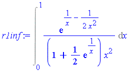
 

> r1inf := Int(-eval(G,v=1/x) * diff(1/x,x), x = 0..1);
 

Int(exp(1/x-1/2/x^2)/((1+1/2*exp(1/x))*x^2), x = 0 .. 1) 

Let the integrand appearing here be named   .  The first few terms of the generalized series expansion of    are as follows. 

> g := op(1,r1inf);
 

exp(1/x-1/2/x^2)/((1+1/2*exp(1/x))*x^2) 


> s := `evalf/int/genseries`(g, x, 6);
 

2*(exp(-1/x^2))^(1/2)/x^2-4*(exp(-1/x^2))^(1/2)*exp(-1/x)/x^2+8*(exp(-1/x^2))^(1/2)*(exp(-1/x))^2/x^2-16*(exp(-1/x^2))^(1/2)*(exp(-1/x))^3/x^2+32*(exp(-1/x^2))^(1/2)*(exp(-1/x))^4/x^2-64*(exp(-1/x^2))...


Maple's symbolic integrator determines that the first two terms of    have the following indefinite integrals. 


> terms := [seq(simplify(op(i,s),symbolic), i=1..6)]:
 

> int(terms[1],x);
 

-Pi^(1/2)*2^(1/2)*erf(1/2*2^(1/2)/x) 

> int(terms[2],x);
 

2*Pi^(1/2)*exp(1/2)*2^(1/2)*erf(1/2*2^(1/2)/x+1/2*2^(1/2)) 

>


Similarly, the integral of each term is computed. 

If we compute the definite integral over  [0, 0.25]  of the successive terms of the generalized series expansion of   , we find that the successive values are as follows. 


> Digits := 2*Digits:
 

> seq( int(terms[i], x=0..0.25), i = 1..6 ):
 

> evalf( [ % ] );
 

[0.15877606054314910751237036266503283736288425513060e-3, -0.47386157552545686895055017987048468405613599844976e-5, 0.146185587516268707710920713064402415368830373380e-6, -0.46204199238888121408794721...
[0.15877606054314910751237036266503283736288425513060e-3, -0.47386157552545686895055017987048468405613599844976e-5, 0.146185587516268707710920713064402415368830373380e-6, -0.46204199238888121408794721...
[0.15877606054314910751237036266503283736288425513060e-3, -0.47386157552545686895055017987048468405613599844976e-5, 0.146185587516268707710920713064402415368830373380e-6, -0.46204199238888121408794721...
[0.15877606054314910751237036266503283736288425513060e-3, -0.47386157552545686895055017987048468405613599844976e-5, 0.146185587516268707710920713064402415368830373380e-6, -0.46204199238888121408794721...
[0.15877606054314910751237036266503283736288425513060e-3, -0.47386157552545686895055017987048468405613599844976e-5, 0.146185587516268707710920713064402415368830373380e-6, -0.46204199238888121408794721...
[0.15877606054314910751237036266503283736288425513060e-3, -0.47386157552545686895055017987048468405613599844976e-5, 0.146185587516268707710920713064402415368830373380e-6, -0.46204199238888121408794721...
[0.15877606054314910751237036266503283736288425513060e-3, -0.47386157552545686895055017987048468405613599844976e-5, 0.146185587516268707710920713064402415368830373380e-6, -0.46204199238888121408794721...
[0.15877606054314910751237036266503283736288425513060e-3, -0.47386157552545686895055017987048468405613599844976e-5, 0.146185587516268707710920713064402415368830373380e-6, -0.46204199238888121408794721...
[0.15877606054314910751237036266503283736288425513060e-3, -0.47386157552545686895055017987048468405613599844976e-5, 0.146185587516268707710920713064402415368830373380e-6, -0.46204199238888121408794721...
[0.15877606054314910751237036266503283736288425513060e-3, -0.47386157552545686895055017987048468405613599844976e-5, 0.146185587516268707710920713064402415368830373380e-6, -0.46204199238888121408794721...
 

>


Clearly, the series representation is rapidly converging on this interval. 

Summing up these values yields the following result for the integral 

of    over  [0, 0.25] . 


> r1 := convert( %, `+` );
 

0.15417915384587540893355973276322641120174289846118e-3


> Digits := 25:
 

>
 

For the remaining interval  [0.25, 1] , ordinary numerical integration methods encounter no difficulties because there are no nearby singularities. 


> r2 := evalf(Int(g, x=0.25..1));
 

.5473062370626801760273993 


Sum these two values to get the integral   . 

> r1inf;
 

Int(exp(1/x-1/2/x^2)/((1+1/2*exp(1/x))*x^2), x = 0 .. 1) 

> r1inf  :=  r1 + r2;
 

.5474604162165260514363329 


Finally, we have obtained the answer for the original integration problem. 


> Int(G, v=0..infinity)  =  r01 + r1inf;
 

Int(exp(v-1/2*v^2)/(1+1/2*exp(v)), v = 0 .. infinity) = 1.305516899118350719237417 

>
 

Multidimensional Numerical Integration 

  • The most significant improvement in numerical integration capabilities for Maple 8 is the addition of numerical methods for multiple integration.
 

  • In previous releases, you could form a multiple integral using nested Int expressions, and then invoke the evalf command on the multiple integration problem. The only solution method was to invoke, recursively, one-dimensional numerical integration methods. This was an inefficient approach to numerical multiple integration problems which would succeed only on the simplest problems.
 

  • In Maple 8, compiled C routines, which implement numerical multiple integration methods, are automatically invoked for such problems whenever the desired precision is in hardware floating-point range (typically about 15 decimal digits).
 

Special (List) Syntax for Multiple Integrals 

  • A numerical multiple integration problem can be specified in a natural way using nested one-dimensional integrals, for example,
 

  evalf( Int(...(Int(Int(f, x1=a1..b1), x2=a2..b2), ...), xn=an..bn) )      

  • where the integrand f depends on x1, x2, ..., xn. Such a problem can also be specified using the following special multiple integration notation with a list as the second argument.
 

  evalf( Int(f, [x1=a1..b1, x2=a2..b2, ..., xn=an..bn])     


  • Additional optional arguments can be stated just as in the case of 1-D integration. Also as in 1-D integration, the integrand f can be specified as a procedure in which case the second argument must be a list of ranges: [a1..b1, a2..b2, ..., an..bn].
 

  • Whether a multiple integration problem is stated using nested integrals or using the list notation, the arguments are extracted so as to invoke the same numerical multiple integration routines.
 

  • See evalf/int for further details and for examples.
 

Example 6: Multidimensional integration 


Multiple integrals may be expressed as nested one-dimensional integrals.  


> restart;
 

> Int(Int(Int(exp(x+y+z)/((5*x+1)*(10*y+2)*(15*z+3)),
                                     x=0..4), y=0..3), z=0..sqrt(2));
 

Int(Int(Int(exp(x+y+z)/((5*x+1)*(10*y+2)*(15*z+3)), x = 0 .. 4), y = 0 .. 3), z = 0 .. 2^(1/2)) 

> evalf(%);
 

.9331611325 


Numerical multiple integration may also be invoked using a list syntax.  


> d := (1 - w^2*x^2*y^2*z^2):
g := d * cos(w*x*y*z) - d * w*x*y*z * sin(w*x*y*z);
 

(1-w^2*x^2*y^2*z^2)*cos(w*x*y*z)-(1-w^2*x^2*y^2*z^2)*w*x*y*z*sin(w*x*y*z)
 

> DesiredIntegral := Int(Int(Int(Int(g, w=0..1), x=0..1), y=0..1), z=0..1);
 

Int(Int(Int(Int((1-w^2*x^2*y^2*z^2)*cos(w*x*y*z)-(1-w^2*x^2*y^2*z^2)*w*x*y*z*sin(w*x*y*z), w = 0 .. 1), x = 0 .. 1), y = 0 .. 1), z = 0 .. 1)


Here we use a list syntax to give the integration command, which would avoid the need to form the nested integral above. 

> evalf(Int(g, [w=0..1, x=0..1, y=0..1, z=0..1]));
 

.9717798177 


Equivalently, we could have requested numerical evaluation of the nested integral formed above. 

> evalf(DesiredIntegral);
 

.9717798177 


When low accuracy is sufficient, the Monte Carlo method may be used.  


> h := 1/(2 + sin(Pi*sqrt(87)*(x1+x2+x3+x4+x5+x6)));
 

1/(2+sin(Pi*87^(1/2)*(x1+x2+x3+x4+x5+x6))) 

> evalf(Int(h, [x1=-1..1, x2=-1..1, x3=-1..1, x4=-1..1, x5=-1..1, x6=-1..1],
            method=_MonteCarlo, epsilon=0.5e-2)):


Only trust about 3 digits when epsilon = 0.5e-2 .  


> evalf[3](%);
 

36.9 

>


Bibliography 

[Bronstein90a]  M. Bronstein, The transcendental Risch differential equation. Journal of Symbolic Computation 9, 1990, pp. 49-60. 


[Bronstein90b]  M. Bronstein, On the integration of elementary functions. Journal of Symbolic Computation 9, 1990, pp. 117-173. 


[Bronstein97]  M. Bronstein, Symbolic Integration I: Transcendental Functions. Springer-Verlag, Berlin, 1997. 


[Cherry85]  G. Cherry, Integration in Finite Terms with Special Functions: the Error Function. Journal of Symbolic Computation 1, 1985, pp. 283-302. 


[Cherry86]  G. Cherry, Integration in Finite Terms with Special Functions: the Logarithmic Integral. SIAM Journal on Computing 15, 1986, pp. 1-21. 


[Cox92]  D. Cox, J. Little and D. O'Shea, Ideals, Varieties, and Algorithms: An Introduction to Computational Algebraic Geometry and Commutative Algebra. Springer-Verlag, New York, 1992. 


[Geddes86]  K.O. Geddes, Numerical integration in a symbolic context. Proceedings of SYMSAC'86, B.W. Char (ed.), ACM Press, New York, 1986, pp. 185-191. 


[Geddes90]  K.O. Geddes, M.L. Glasser, R.A. Moore and T.C. Scott, Evaluation of classes of definite integrals involving elementary functions via differentiation of special functions. Applicable Algebra in Engineering, Communication and Computing 1 (2), 1990, pp. 149-165. 


[Geddes92]  K.O. Geddes, S.R. Czapor and G. Labahn, Algorithms for Computer Algebra. Kluwer Academic Publishers, Boston, 1992. 


[GeddesFee92]  K.O. Geddes and G.J. Fee, Hybrid symbolic-numeric integration in Maple.  Proceedings of ISSAC'92, P.S. Wang (ed.), ACM Press, New York, 1992, pp. 36-41. 


[GeddesGonnet89]  K.O. Geddes and G.H. Gonnet, A new algorithm for computing symbolic limits using hierarchical series. Appears in Symbolic and Algebraic Computation, P. Gianni (ed.), Lecture Notes in Computer Science, No. 358, Springer-Verlag, Berlin, 1989, pp. 490-495. 


[Jeffrey93]  D.J. Jeffrey, Integration to obtain expressions valid on domains of maximum extent. Proceedings of ISSAC'93, M. Bronstein (ed.), ACM Press, New York, 1993, pp. 34-41. 


[Jeffrey97]  D.J. Jeffrey, Rectifying transformations for the integration of rational trigonometric functions. Journal of Symbolic Computation 24, 1997, pp. 563-573. 


[PBM90]  A.P. Prudnikov, Y. Brychkov and O. Marichev, Integrals and Series, Volume 3: More Special Functions. Gordon and Breach Science Publishers, 1990. 


[Richardson96]  D. Richardson, B. Salvy, J. Shackell and J. Van derHoeven, Asymptotic expansions of exp-log functions. Proceedings of ISSAC'96, Y.N. Lakshman (ed.), ACM Press, New York, 1996, pp. 309-313. 


[Roach96]  K.B. Roach, Hypergeometric Function Representations. Proceedings of ISSAC '96, Y.N. Lakshman (ed.), ACM Press, New York, 1996, pp 301-308. 


[Roach97]  K.B. Roach, Meijer G Function Representations. Proceedings of ISSAC '97, W.W. Kuechlin (ed.), ACM Press, New York, 1997, pp. 205-211.
 

[Salvy91]  B. Salvy, Examples of automatic asymptotic expansions. SIGSAM Bulletin 25 (2), 1991, pp. 4-17. 


[Salvy92]  B. Salvy, General asymptotic scales and computer algebra. Appears in Asymptotic and Numerical Methods for Partial Differential Equations, Critical Parameters and Domain Decomposition, H. Kaper and M. Garbey (ed.), Kluwer Academic Publishers, 1992, pp. 255-266. 


[Trager84]  B.M. Trager, On the integration of algebraic functions. Ph.D. Thesis, Computer Science, MIT, 1984.
 

>