Given a prior distribution $Pr(X)$ over variables $X$ of interest, representing degrees of belief, and given new evidence $E = e$ for some variable $E$, revise your degrees of belief: posterior $Pr(X|E = e)$.
Issue
How do we specify the full joint distribution over a set of random
variables $X_1, X_2, \dots, X_n$?
Exponential number of possible worlds
e.g., if $X_i$ is Boolean, then $2^n$ numbers (or $2^n - 1$ parameters, since they sum to 1)
These numbers are not robust/stable
Inference is frightfully slow
Must sum over exponential number of worlds to answer queries
Independence
X and Y are independent iff: $\forall x \in dom(X), y \in dom(Y)$
$Pr (X = x) = Pr(X = x | Y = y)$
$Pr(X = x, Y = y) = Pr(X = x)Pr(Y = y)$
Intuitively, learning the value of $Y$ doesn't influence our beliefs about $X$ and vice versa.
Conditional Independence
Two variables $X$ and $Y$ are conditionally independent given variable $Z$ iff: $\forall x \in dom(X), y \in dom(Y), z \in dom(Z)$
$Pr(X = x|Z = z) = Pr(X = x|Y = y, Z = z)$
$Pr(X = x, Y = y| Z = z) = Pr(X = x|Z = z) Pr(Y = y|Z = z)$
If you know the value of $Z$ (whatever it is), nothing you learn about $Y$ will influence your beliefs about $X$
We can specify full joint distribution using only $n$ parameters (linear) instead of $2^n - 1$ (exponential)
Simply specify $Pr(x_1) , \dots , Pr(x_n)$.
Lecture 6: Bayesian Networks
Bayesian Networks (BN)
Graphical representation of the direct dependencies over a set of variables + a set of conditional probability tables (CPTs) quantifying the strength of those influences.
A BN over variables $\{X_1, X_2, \dots, X_n\}$
consists of:
a DAG whose nodes are the variables
a set of CPTs ($Pr(X_i | Parents(X_i)$) for each $X_i$
Also known as
Belief networks
Probabilistic networks
Key notions
parents of a node: $Par(X_i)$
children of node
descendants of a node
ancestors of a node
family: set of nodes consisting of $X_i$ and its parents
CPTs are defined over families in the BN
Semantics of a Bayes Net
The structure of the BN means: every $X_i$ is conditionally independent of all of its non-descendants given its parents:
$Pr(X_i | S \cup Par(X_i)) = Pr(X_i | Par(X_i))$ for any subset $S \subseteq NonDescendants(X_i)$
The joint is recoverable using the parameters (CPTs)
specified in an arbitrary BN
Constructing a Bayes Net
Given any distribution over variables $X_1, X_2, \dots , X_n$, we can construct a Bayes net that faithfully represents that distribution.
Take any ordering of the variables (say, the order given), and go through the following procedure for $X_n$ down to $X_1$.
Let $Par(X_n)$ be any subset $S \subseteq \{X_1, \dots , X_{n-1}\}$ such that $X_n$ is independent of
$\{X_1, \dots, X_{n-1}\} - S$ given $S$. Such a subset must exist (convince yourself).
Then determine the parents of $X_{n-1}$ in the same way, finding a similar $S \subseteq \{X_1, \dots, X_{n - 2}\}$, and so on.
In the end, a DAG is produced and the BN semantics must hold by construction.
Causal Intuitions
The construction of a BN is simple
works with arbitrary orderings of variable set
but some orderings are much better than others!
generally, if ordering/dependence structure reflects causal intuitions, a more natural, compact BN results
Testing Independence
Given a BN, how can we test whether two variables $X$ and $Y$ are independent (given evidence $E$)?
D-separation
A set of variables $E$ d-separates $X$ and $Y$ if it blocks every undirected path in the BN between $X$ and $Y$.
$X$ and $Y$ are conditionally independent given evidence $E$ if $E$ d-separates $X$ and $Y$
The algorithm, variable elimination, simply applies the summing out rule repeatedly.
Factors
A function $f(X_1, X_2, \dots, X_k)$ is also called a factor. We can view this as a table of numbers, one for each instantiation of the variables $X_1, X_2, \dots, X_k$.
Notation: $f(\mathbf{X},\mathbf{Y})$ denotes a factor over the variables $\mathbf{X} \cup \mathbf{Y}$. (Here $\mathbf{X}, \mathbf{Y}$ are sets of variables.)
The Product of Two Factors
Summing a Variable Out of a Factor
Restricting a Factor
Relevance: A Sound Approximation
We can restrict attention to relevant variables. Given query $Q$, evidence $\mathbf E$:
$Q$ is relevant
if any node $Z$ is relevant, its parents are relevant
if $E \in \mathbf E$ is a descendent of a relevant node, then $E$ is relevant
We can restrict our attention to the subnetwork comprising only relevant variables when evaluating a query Q
Lecture 8: Causal Inference
Causality
Causality is the study of how things influence one other, how causes lead to effects.
Causal dependence: $X$ causes $Y$ iff changes to $X$ induce changes to $Y$
Causal and Non-Causal Correlations
A joint distribution $P(X, Y)$ captures correlations between $X$ and $Y$, but does not indicate whether a causal relation exists between $X$ and $Y$ nor
the direction of the causal relation when it exists.
A conditional distribution $P(Y|X)$ does not necessarily indicate $X$ causes $Y$.
Causal Bayesian Network
Definition: Bayesian network where all edges indicate direct causal effects.
Causal Inference
Intervention: What is the effect of an action?
Causal networks can easily support intervention queries,
but not non-causal networks do not.
Inference with Do Operator
$$P(X | do(Y = y), Z = z)$$
In a causal graph:
Remove edges pointing to $Y$ and $P(Y|parents(Y))$
Perform variable elimination on remaining graph:
Restrict factors to evidence: $Y = y$ and $Z = z$
Eliminate variables
Multiply remaining factors and normalize
Counterfactual Analysis
Counterfactual analysis (or counterfactual thinking): explores outcomes that did not actually occur, but which could have occurred under different conditions. It's a kind of what if? analysis and is a useful way for testing cause-and-effect relationships.
Structural Causal Models
Idea: separate causal relations from noise
Structural Causal Model contains:
$X$: endogenous variables (domain variables)
$U$: exogenous variables (noise)
Only deterministic relations given by equations
$X_i = f(parents(X_i), U_i)$
Conversion
Structural Causal Models (SCMs) can be converted into equivalent Causal Bayesian Network, but not the other way around
SCMs separate causal relations from the noise and therefore provide more information
Can specify entire process with finitely many time slices.
Hidden Markov Models
Problems
States not directly observable, hence uncertainty captured by a distribution
Uncertain dynamics increase state uncertainty
Observations made via sensors reduce state uncertainty
First-order Hidden Markov Model
Definition:
Set of states: $S$
Set of observations: $O$
Transition model: $Pr(s_t|s_{t-1})$
Observation model: $Pr(o_t|s_t)$
Prior: $Pr(s_0)$
Inference in temporal models
Monitoring
$Pr(s_t | o_t, \dots, o_1)$: distribution over current state given observations
Forward algorithm
Prediction
$Pr(s_{t+k} | o_t, \dots, o_1)$: distribution over future state given observations
Forward algorithm
Hindsight
$Pr(s_k | o_t, \dots, o_1)$ for $k < t$: distribution over a past state given observations
Forward-backward algorithm
Most likely explanation
$Argmax_{s_0, \dots, s_t} Pr(s_0, \dots,s_t|o_t, \dots, o_1)$: most likely state sequence given observations
Viterbi algorithm
Complexity of temporal inference
Hidden Markov Models are Bayes nets with a polytree structure
Hence, variable elimination is
Linear with respect to # of time slices
Linear with respect to largest conditional probability table ($Pr(s_t|s_{t-1})$ or $Pr(o_t|s_t)$)
Dynamic Bayesian Networks
Idea: encode states and observations with several random variables
Advantage: exploit conditional independence to save time and space
HMMs are just DBNs with one state variable and one observation
variable
DBN complexity
Conditional independence allows us to write transition and observation models very compactly!
Time and space of inference: conditional independence rarely helps…
Inference tends to be exponential in the number of state variables
Intuition: all state variables eventually get correlated
No better than with HMMs
Non-Stationary Process
What if the process is not stationary?
Solution: add new state components until dynamics are stationary
Non-Markovian Process
What if the process is not Markovian?
Solution: add new state components until dynamics are Markovian
Markovian Stationary Process
Problem: adding components to the state description to force a process to be Markovian and stationary may significantly increase computational complexity
Solution: try to find the smallest state description that is self-sufficient (i.e., Markovian and stationary)
Lecture 10: Decision Tree Learning
What is Machine Learning?
A computer program is said to learn from experience E with respect to some
class of tasks T and performance measure P, if its performance at tasks in T, as
measured by P, improves with experience E. [Tom Mitchell, 1997]
Inductive learning (also known as concept learning)
Given a training set of examples of the form $(x,f(x))$
$x$ is the input, $f(x)$ is the output
Return a function $h$ that approximates $f$
$h$ is called the hypothesis
Hypothesis Space
Hypothesis space $H$
Set of all hypotheses $h$ that the learner may consider
Learning is a search through hypothesis space
Objective
Find hypothesis that agrees with training examples
But what about unseen examples?
Generalization
A good hypothesis will generalize well (i.e., predict unseen examples correctly)
Usually, any hypothesis h found to approximate the target function f well over
a sufficiently large set of training examples will also approximate the
target function well over any unobserved examples
Ockham's razor
Prefer the simplest hypothesis consistent with data
Inductive learning
Finding a consistent hypothesis depends on the hypothesis space
For example, it is not possible to learn exactly f(x)=ax+b+xsin(x) when H=space of polynomials of finite degree
A learning problem is realizable if the hypothesis space contains the true function, otherwise it is unrealizable
Difficult to determine whether a learning problem is realizable since the true function is not known
It is possible to use a very large hypothesis space
For example, H=class of all Turing machines
But there is a tradeoff between expressiveness of a hypothesis class and complexity of finding simple, consistent hypothesis within the space
Fitting straight lines is easy, fitting high degree polynomials is hard, fitting Turing machines is very hard!
Decision trees
Decision tree classification
Nodes: labeled with attributes
Edges: labeled with attribute values
Leaves: labeled with classes
Classify an instance by starting at the root, testing the
attribute specified by the root, then moving down the
branch corresponding to the value of the attribute
Continue until you reach a leaf
Return the class
Decision trees can represent disjunctions of conjunctions of constraints on attribute values
Decision tree representation
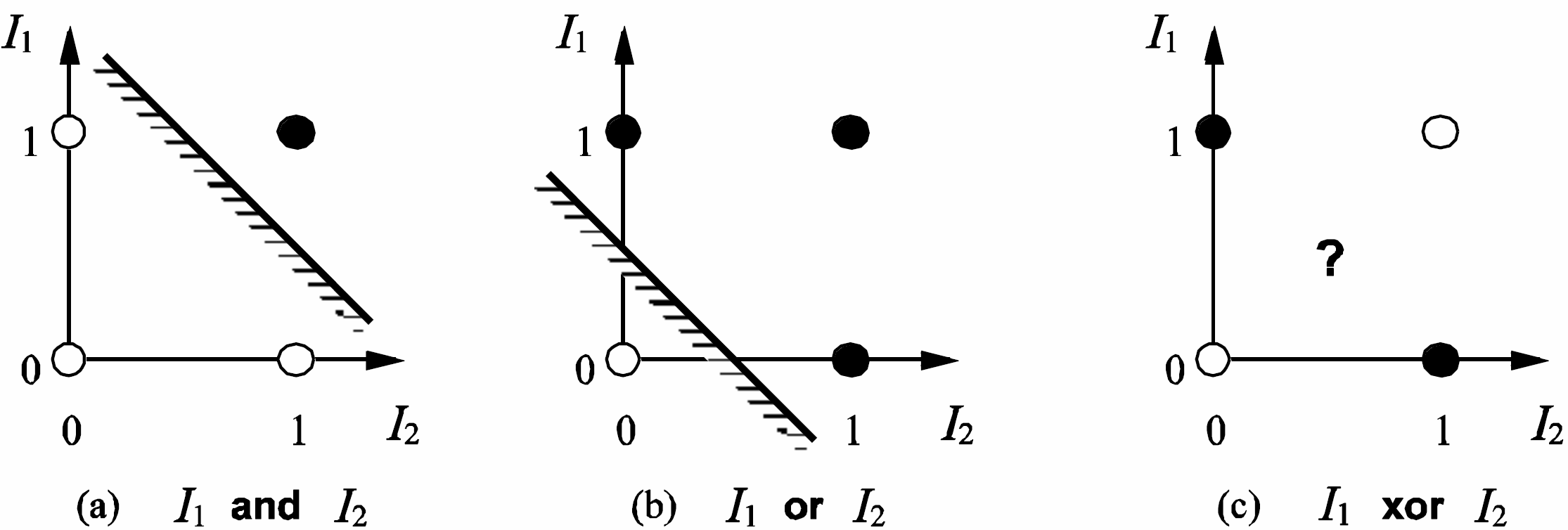
Decision trees are fully expressive within the class of propositional languages
Any Boolean function can be written as a decision tree
Trivially by allowing each row in a truth table correspond to a path in the tree
Can often use small trees
Some functions require exponentially large trees (majority function, parity function)
However, there is no representation that is efficient for all functions
Inducing a decision tree
Aim: find a small tree consistent with the training examples
Idea: (recursively) choose "most significant" attribute as root of (sub)tree
Choosing attribute tests
The central choice is deciding which attribute to test at each node
We want to choose an attribute that is most useful for classifying examples
Idea: a good attribute splits the examples into subsets that are (ideally) "all positive" or "all negative"
Using information theory
Measure uncertainty (Entropy):
$$I(P(v_1), \dots, P(v_n)) = \sum_{i = 1}^n -P(v_i) \log_2 P(v_i)$$
For a training set containing $p$ positive examples and $n$ negative examples:
$$I(\frac{p}{p+n}, \frac{n}{p+n}) = -\frac{p}{p+n} \log_2 \frac{p}{p+n} - \frac{n}{p+n} \log_2 \frac{n}{p+n}$$
Information gain
A chosen attribute $A$ divides the training set $E$ into subsets $E_1, \dots , E_v$ according to their values for $A$, where $A$ has $v$ distinct values.
$$remainder(A) = \sum_{i = 1}^v \frac{p_i + n_i}{p + n} I\left( \frac{p_i}{p_i + n_i}, \frac{n_i}{p_i + n_i} \right)$$
Information Gain (IG) or reduction in uncertainty from the attribute test:
$$IG(A) = I\left( \frac{p}{p + n}, \frac{n}{p + n} \right) - remainder(A)$$
Choose the attribute with the largest IG
Performance of a learning algorithm
A learning algorithm is good if it produces a hypothesis that does a good job of predicting classifications of unseen examples
Verify performance with a test set
Collect a large set of examples
Divide into 2 disjoint sets: training set and test set
Learn hypothesis h with training set
Measure percentage of correctly classified examples by h in the test set
Overfitting
Given a hypothesis space $H$, a hypothesis $h \in H$ is said to overfit the training data if there exists some alternative hypothesis $h' \in H$ such that $h$ has smaller error than $h'$ over the training examples but $h'$ has smaller error than $h$ over the entire distribution of instances
Overfitting can decrease accuracy of decision trees by 10-25%
Avoiding overfitting
Two popular techniques:
Prune statistically irrelevant nodes
Measure irrelevance with $\chi^2$ test
Ideally: stop growing tree when test set performance decreases
Use cross-validation
Choosing Tree Size
Problem: since we are choosing Tree Size based on the test set, the test set effectively becomes part of the training set when optimizing Tree Size. Hence, we cannot trust anymore the test set accuracy to be representative of future accuracy.
Solution: split data into training, validation and test sets
Training set: compute decision tree
Validation set: optimize hyperparameters such as Tree Size
Test set: measure performance
Robust validation
How can we ensure that validation accuracy is representative of future accuracy?
Validation accuracy becomes more reliable as we increase the size of the validation set
However, this reduces the amount of data left for training
Popular solution: cross-validation
Cross-Validation
Repeatedly split training data in two parts, one for training and one for validation. Report the average validation accuracy.
$k$-fold cross validation: split training data in $k$ equal size subsets. Run $k$ experiments, each time validating on one subset and training on the remaining subsets. Compute the average validation accuracy of the $k$ experiments.
Lecture 11: Statistical Learning
Statistical Learning
View: we have uncertain knowledge of the world
Idea: learning simply reduces this uncertainty
Bayesian Learning
Prior: $Pr(H)$
Likelihood: $Pr(d|H)$
Evidence: $\mathbf d = \langle d_1,d_2,\dots,d_n \rangle$
Bayesian Learning amounts to computing the posterior using Bayes' Theorem: $$Pr(H|\mathbf d) = k Pr(\mathbf d|H)Pr(H)$$
Bayesian Prediction
Suppose we want to make a prediction about an unknown quantity X (i.e., the flavor of the next candy)
Error function
\[E(\mathbf{W}) = \frac{1}{2} \sum_{n} E_n(\mathbf{W}) = \frac{1}{2} \sum_{n} || f(\boldsymbol{x_n}, \mathbf{W}) - y_n||_2^2 \]
where \(\mathbf{x_n}\) is the input of the \(n^{th}\) example, \(y_n\) is the label of the \(n^{th}\) example, \(f(\boldsymbol{x_n}, \mathbf{W})\) is the output of the neural net.
Sequential Gradient Descent
For each example \(\boldsymbol{x}_n, y_n\) adjust the weights as follows:
\[w_{ji} \leftarrow w_{ji} - \eta \frac{\partial E_n}{\partial w_{ji}}\]
How can we compute the gradient efficiently given an arbitrary network structure?
Answer: backpropagation algorithm
Today: automatic differentiation
Backpropagation Algorithm
Two phases:
Forward phase: compute output \(z_j\) of each unit \(j\)
Backward phase: compute delta \(\delta_j\) at each unit \(j\)
Forward phase
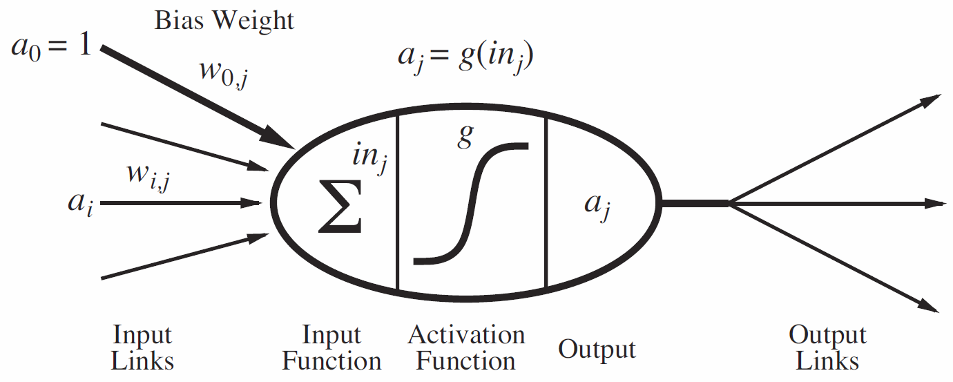
Propagate inputs forward to compute the output of each unit
Output \(z_j\) at unit \(j\):
\(z_j = h(a_j)\) where \(a_j = \sum_i w_{ji} z_i\)
Backward phase
Use chain rule to recursively compute gradient
For each weight \(w_{ji}\): \(\frac{\partial E_n}{\partial w_{ji}} = \frac{\partial E_n}{\partial a_j} \frac{\partial a_j}{\partial w_{ji}} = \delta_j z_i\)
Let \(\delta_j \equiv \frac{\partial E_n}{\partial a_j}\) then
\[\delta_j = \begin{cases}
h'(a_j) (z_j - y_j) & \text{base case: \(j\) is an output unit} \\
h'(a_j) \sum_k w_{kj} \delta_k & \text{recursive case: \(j\) is an hidden unit}
\end{cases}\]
Since \(a_j = \sum_{i} w_{ji} z_i\), then \(\frac{\partial a_j}{\partial w_{ji}} = z_i\).
Simple Example Using \(\tanh(x)\)
Please refer to the notes...
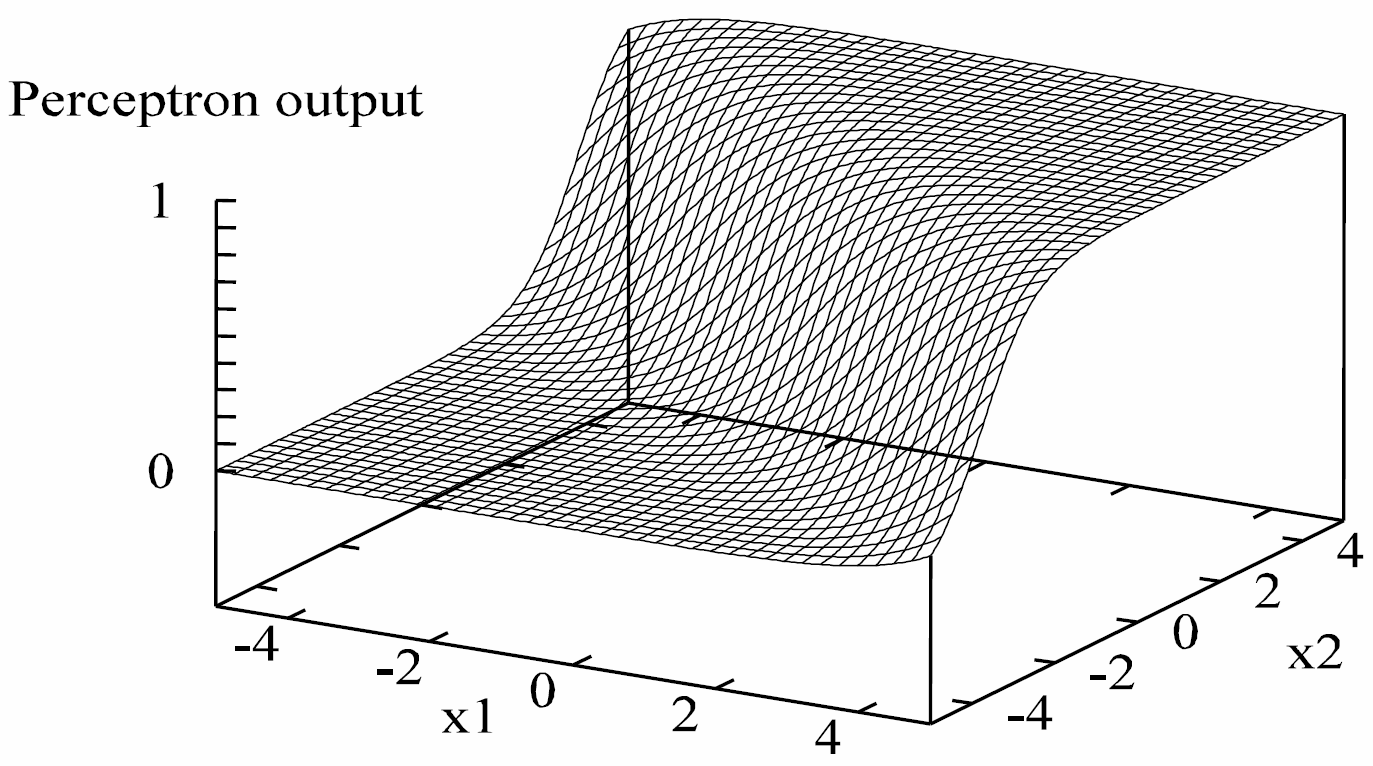
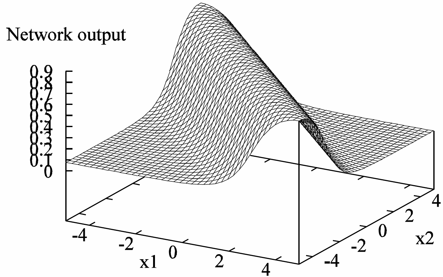
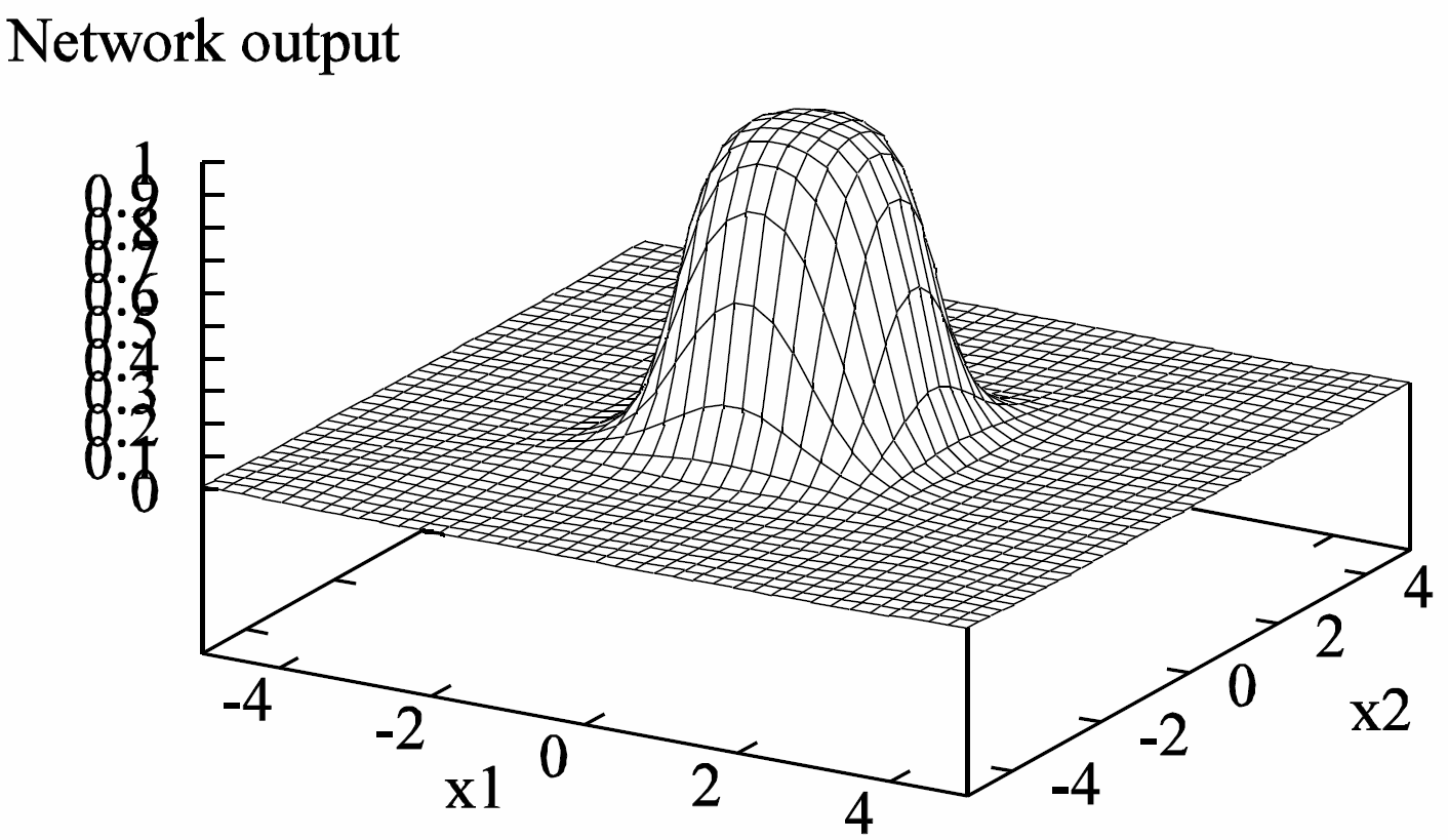
Non-linear regression examples
Two-layer network:
3 tanh hidden units and 1 identity output unit
Analysis
Efficiency:
Fast gradient computation: linear in number of weights
Convergence:
Slow convergence (linear rate)
May get trapped in local optima
Prone to overfitting
Solutions: early stopping, regularization (add \(||w||_2^2\) penalty term to objective), dropout
Lecture 14: Deep Neural Networks
Deep Neural Networks
Definition: neural network with many hidden layers
Advantage: high expressivity
Challenges:
How should we train a deep neural network?
How can we avoid overfitting?
Expressiveness
Neural networks with one hidden layer of sigmoid/hyperbolic units can approximate arbitrarily closely neural networks with several layers of sigmoid/hyperbolic units
However as we increase the number of layers, the number of units needed may decrease exponentially (with the number of layers)
Vanishing Gradients
Deep neural networks of sigmoid and hyperbolic units often suffer from vanishing gradients
Avoiding Vanishing Gradients
Several popular solutions:
Pre-training
Rectified linear units
Skip connections
Batch normalization
Rectified Linear Units
Rectifier (ReLU): \(h(a) = \max(0, a)\)
Gradient is 0 or 1
Sparse computation
Soft version (“Softplus”) : \(h(a) = \log(1 + e^a)\)
Warning: softplus does not prevent gradient vanishing (gradient < 1)
Overfitting
High expressivity increases the risk of overfitting
# of parameters is often larger than the amount of data
Some solutions:
Regularization
Dropout
Data augmentation
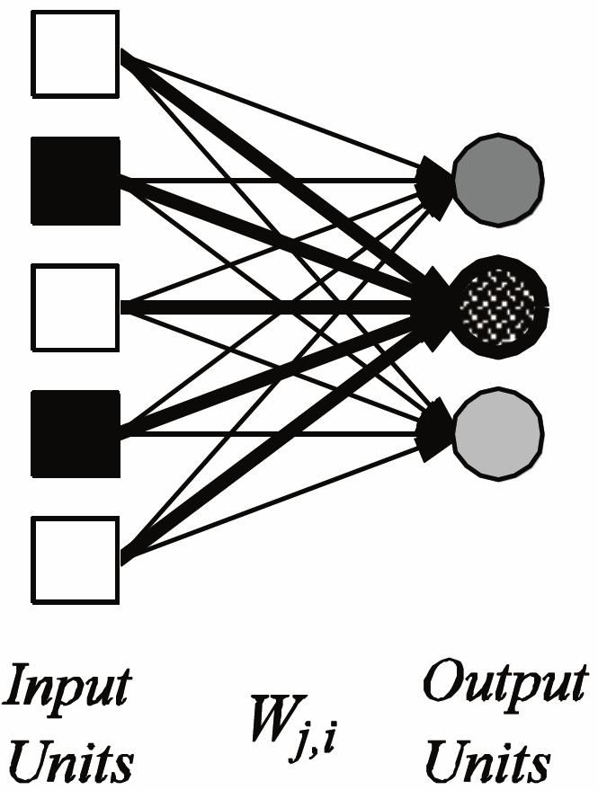
Dropout
Idea: randomly “drop” some units from the network when training
Training: at each iteration of gradient descent
Each input unit is dropped with probability \(p_1\) (e.g., 0.2)
Each hidden unit is dropped with probability \(p_2\) (e.g., 0.5)
Prediction (testing):
Multiply each input unit by \(1 - p_1\)
Multiply each hidden unit by \(1 - p_2\)
Intuition
Dropout can be viewed as an approximate form of ensemble learning
In each training iteration, a different subnetwork is trained
At test time, these subnetworks are “merged” by averaging their weights
Lecture 15: Decision Networks
Preferences
A preference ordering \(\succcurlyeq\) is a ranking of all possible states of affairs (worlds) S
these could be outcomes of actions, truth assignments, states in a search problem, etc.
\(s \succcurlyeq t\): means that state s is at least as good as t
\(s \succ t\): means that state s is strictly preferred to t
\(s \sim t\): means that the agent is indifferent between states s and t
If an agent's actions are deterministic then we know what states will occur
If an agent's actions are not deterministic then we represent this by lotteries
Probability distribution over outcomes
Lottery \(L=[p_1,s_1; p_2,s_2; \dots; p_n,s_n]\)
\(s_1\) occurs with probability \(p_1\), \(s_2\) occurs with probability \(p_2\), ...
Axioms
Orderability: Given 2 states A and B
\[(A \succ B) \vee (B \succ A) \vee (A \sim B)\]
Transitivity: Given 3 states, A, B, and C
\[(A \succ B) \wedge (B \succ C) \Rightarrow (A \succ C)\]
Continuity:
\[A \succ B \succ C \Rightarrow \exists p \quad [p, A; 1-p, C] \sim B\]
Substitutability:
\[A \sim B \Rightarrow [p, A ; 1 - p, C] \sim [p, B; 1 - p, C]\]
Monotonicity:
\[A \succ B \Rightarrow \left( p \geq q \Leftrightarrow [p, A; 1 - p, B] \succ [q, A; 1 - q, B] \right)\]
Structure of preference ordering imposes certain “rationality requirements” (it is a weak ordering)
Utilities
Instead of ranking outcomes, we quantify our preferences
e.g., how much more valuable is coffee than tea
A utility function \(U: S \to \mathbb R\) associates a real-valued utility with each outcome.
\(U(s)\) measures your degree of preference for \(s\)
Note: \(U\) induces a preference ordering \(\succcurlyeq_U\) over \(S\) defined as: \(s \succcurlyeq_U t\) iff \(U(s) \geq U(t)\)
obviously \(\succcurlyeq_U\) will be reflexive and transitive
Expected Utility
Under conditions of uncertainty, each decision \(d\) induces a distribution \(Pr_d\) over possible outcomes
\(Pr_d(s)\) is probability of outcome \(s\) under decision \(d\)
The expected utility of decision \(d\) is defined
\[EU(d) = \sum_{s \in S} Pr_d(s) U(s)\]
The principle of maximum expected utility (MEU) states that the optimal decision under conditions of uncertainty is that with the greatest expected utility.
Decision Networks
Decision networks (also known as influence diagrams) provide a way of representing sequential decision problems
basic idea: represent the variables in the problem as you would in a Bayesian network
add decision variables – variables that you “control”
add utility variables – how good different states are
Chance Nodes
random variables, denoted by circles
as in a BN, probabilistic dependence on parents
Decision Nodes
variables set by decision maker, denoted by squares
parents reflect information available at time decision is to be made
Value node
specifies utility of a state, denoted by a diamond
utility depends only on state of parents of value node
generally: only one value node in a decision network
Assumptions
Decision nodes are totally ordered
decision variables D1, D2, ..., Dn
decisions are made in sequence
e.g., BloodTst (yes,no) decided before Drug (fd,md,no)
No-forgetting property
any information available when decision Di is made is available when decision Dj is made (for i < j)
thus all parents of Di are parents of Dj
Policies
Let \(Par(D_i)\) be the parents of decision node \(D_i\)
\(Dom(Par(D_i))\) is the set of assignments to parents
A policy \(\delta\) is a set of mappings \(\delta_i\), one for each decision node \(D_i\)
\(\delta_i :Dom(Par(D_i)) \to Dom(D_i)\)
\(\delta_i\) associates a decision with each parent asst for \(D_i\)
Value of a Policy
Value of policy \(\delta\) is the expected utility given that decisions are executed according to \(\delta\)
Given asst \(x\) to the set \(X\) of all chance variables, let
\(\delta(x)\) denote the asst to decision variables dictated by \(\delta\)
e.g., asst to D1 determined by it's parents' asst in \(x\)
e.g., asst to D2 determined by it's parents' asst in \(x\) along with whatever was assigned to D1
Value of \(\delta : EU(\delta) = \sum_{X} P(X, \delta (X)) U(X, \delta(X))\)
Optimal Policies
An optimal policy is a policy \(\delta^*\) such that \(EU(\delta^*) \geq EU(\delta)\) for all policies
We can use the dynamic programming principle yet again to avoid enumerating all policies
We can also use the structure of the decision network to use variable elimination to aid in the computation
Optimizing Policies: Key Points
If a decision node \(D\) has no decisions that follow it, we can find its policy by instantiating each of its parents and computing the expected utility of each decision for each parent instantiation
no-forgetting means that all other decisions are instantiated (they must be parents)
its easy to compute the expected utility using VE
the number of computations is quite large: we run expected utility calculations (VE) for each parent instantiation together with each possible decision D might allow
policy: choose max decision for each parent instant’n
When a decision D node is optimized, it can be treated as a random variable
for each instantiation of its parents we now know what value the decision should take
just treat policy as a new CPT: for a given parent instantiation x, D gets (x) with probability 1 (all other decisions get probability zero)
If we optimize from last decision to first, at each point we can optimize a specific decision by (a bunch of) simple VE calculations
it’s successor decisions (optimized) are just normal nodes in the BNs (with CPTs)
Instead of evaluating the state value function, \(V^π(s)\), evaluate the state-action value function, \(Q^π(s,a)\)
\(Q^π(s,a)\) : value of executing \(a\) followed by \(\pi\)
\[Q^\pi(s, a) = \mathbb E[r | s, a] + \gamma \sum_{s'} Pr(s' | s, a) V^\pi(s')\]
Convergence of Linear Function Approximation Q-Learning
Linear Q-Learning converges under the same conditions as Tabular Q-learning.
Divergence of Non-linear Gradient Q-learning
Even when the following conditions hold
\(\sum_{t = 0}^\infty \alpha_t = \infty\) and \(\sum_{t = 0}^{\infty} \alpha_t^2 < \infty\) non-linear Q-learning may diverge
Intuition:
Adjusting \(w\) to increase \(Q\) at \((s, a)\) might introduce errors at nearby state-action pairs.
Mitigating divergence
Two tricks are often used in practice:
Experience replay
Use two networks:
Q-network
Target network
Experience Replay
Idea: store previous experiences \(\langle s, a, s', r \rangle\) into a buffer and sample a mini-batch of previous experiences at each step to learn by Q-learning
Advantages
Break correlations between successive updates (more stable learning)
Less interactions with environment needed (better data efficiency)
Target Network
Idea: Use a separate target network that is updated only periodically
repeat for each \((s, a, s', r)\) in mini-batch:
Advantage: mitigate divergence
Similar to value iteration.
Check the course notes for formula.
Deep Q-network (DQN)
Check the course notes for pseudocode.
Lecture 19: Model-based Reinforcement Learning
Model-free Online RL
No explicit transition or reward models
Q-learning: value-based method
Policy gradient: policy-based method
Actor critic: policy and value-based method
Model-based Online RL
Learn explicit transition and/or reward model
Plan based on the model
Benefit: Increased sample efficiency
Drawback: Increased complexity
Model-based RL
Idea: at each step
Execute action
Observe resulting state and reward
Update transition and/or reward model
Update policy and/or value function
Model-based RL (with Value Iteration)
Please check the course notes for pseudocode.
Partial Planning
In complex models, fully optimizing the policy or value function at each time step is intractable
Consider partial planning
A few steps of Q-learning
Learning from simulated experience
Model-based RL (with Q-learning)
Please check the course notes for pseudocode.
Partial Planning vs Replay Buffer
Previous algorithm is very similar to Model-free Q-learning with a replay buffer
Instead of updating Q-function based on samples from replay buffer, generate samples from model
Replay buffer:
Simple, real samples, no generalization to other state-action pairs
Partial planning with a model
Complex, simulated samples, generalization to other state-action pairs (can help or hurt)
Dyna
Learn explicit transition and/or reward model
Plan based on the model
Learn directly from real experience
Dyna-Q
Please check the course notes for pseudocode.
Planning from Current State
Instead of planning at arbitrary states, plan from the current state
This helps improve next action
Monte Carlo Tree Search
Tractable Tree Search
Combine 3 ideas:
Leaf nodes: approximate leaf values with value of default policy
\[Q^*(s, a) \approx Q^{\pi}(s, a) \approx \frac{1}{n(s, a)} \sum_{k = 1}^n G_k\]
Chance nodes: approximate expectation by sampling from transition model
\[Q^*(s, a) \approx R(s, a) + \gamma \sum_{s' \sim Pr(s' | s, a)} V(s')\]
Decision nodes: expand only most promising actions
\[a^* = \arg \max_a Q(s, a) + c \sqrt{\frac{2 \ln{n(s)}}{n(s, a)}}\] and
\[V^*(s) = \max_{a^*} Q^*(s, a^*)\]
Resulting algorithm: Monte Carlo Tree Search
Monte Carlo Tree Search (with upper confidence bound)
Please check the course notes for pseudocode.
Monte Carlo Tree Search (continued)
Please check the course notes for pseudocode.
Monte Carlo Tree Search (continued)
Please check the course notes for pseudocode.
AlphaGo
Four steps:
Supervised Learning of Policy Networks
Policy gradient with Policy Networks
Value gradient with Value Networks
Searching with Policy and Value Networks
Monte Carlo Tree Search variant
Search Tree
At each edge store \(Q(s, a), \pi(a | s), n(s, a)\)
Where \(n(s, a)\) is the visit count of \((s, a)\)
Simulation
At each node, select edge \(a^*\) that maximizes
\[a^* = \arg \max_a Q(s, a) + u(s, a)\]
where \(u(s, a) \propto \frac{\pi(a | s)}{1 + n(s, a)}\) is an exploration bonus
\[Q(s, a) = \frac{1}{n(s, a)} \sum_{i} \mathbb 1_i(s, a) \left[ \lambda V_w(s) + (1 - \lambda) G_i \right] \]
\[\mathbb 1_i(s, a) = \begin{cases}
1 & \text{if } \text{simulation } i \text{ visits } (s, a) \\
0 & \text{otherwise}
\end{cases}\]
Lecture 20: Multi-Armed Bandits
Exploration/Exploitation Tradeoff
Fundamental problem of RL due to the active nature of the learning process
Consider one-state RL problems known as bandits
Stochastic Bandits
Formal definition:
Single state: \(S = \{s\}\)
\(A\): set of actions (also known as arms)
Space of rewards (often re-scaled to be [0,1])
Finite/Infinite horizons
Average reward setting (\(\gamma = 1\))
No transition function to be learned since there is a single state
We simply need to learn the stochastic reward function
Simple Heuristics
Greedy strategy: select the arm with the highest average so far
May get stuck due to lack of exploration
\(\epsilon\)-greedy: select an arm at random with probability \(\epsilon\) and otherwise do a greedy selection
Convergence rate depends on choice of \(\epsilon\)
Regret
Let \(R(a)\) be the true (unknown) expected reward of \(a\)
Let \(r^* = \max_a R(a)\) and \(a^* = \arg \max_a R(a)\)
Denote by \(loss(a)\) the expected regret of \(a\)
Denote by \(Loss_n\) the expected cumulative regret for \(n\) time steps
\[Loss_n = \sum_{t = 1}^n loss(a_t)\]
Theoretical Guarantees
When \(\epsilon\) is constant, then
For large enough \(t\): \(Pr(a_t \neq a^*) \approx \epsilon\)
But \(R(a) \geq R(a'), \forall a'\) contradicts our assumption that \(a\) is suboptimal.
Probabilistic Upper Bound
Problem: We can't compute an upper bound with certainty since we are sampling
However we can obtain measures that are upper bounds most of the time
i.e., \(Pr(R(a) \leq f(a)) \geq 1 - \delta\)
Example: Hoeffding's inequality
\[Pr\left( R(a) \leq \tilde R(a) + \sqrt{\frac{\log(1/\delta)}{2n_a}} \right) \geq 1 - \delta\]
where \(n_a\) is the number of trials of arm \(a\)
Upper Confidence Bound (UCB)
Set \(\delta_n = 1/n^4\) in Hoeffding's bound
Choose \(a\) with highest Hoeffding bound
Please check the course notes for pseudocode.
UCB Convergence
Theorem: Although Hoeffding’s bound is probabilistic, UCB converges.
Idea: As \(n\) increases, the term \(\sqrt{\frac{2\log(n)}{n_a}}\) increases, ensuring that all arms are tried infinitely often
Distribution over next reward \(r^a\)
\[Pr(r^a_{n + 1} | r_1^a, r_2^a, \dots, r_n^a) = \int_\theta Pr(r^a_{n + 1} | \theta) Pr(\theta | r_1^a, r_2^a, \dots, r_n^a) d\theta\]
Distribution over \(R(a)\) when \(\theta\) includes the mean
\[Pr(R(a) | r_1^a, r_2^a, \dots, r_n^a) = Pr (\theta | r_1^a, r_2^a, \dots, r_n^a)\]
if \(\theta = R(a)\)
A dominant strategy dominates all other strategies
A rational agent will never play a dominated strategy
Each player may or may not have dominant strategy
When each player has a dominant strategy, the set of those strategies (strategy profile) is a dominant strategy equilibrium (DSE)
DSE: \(\{\sigma_1, \dots, \sigma_N\}\) if \(\sigma_i\), for all \(i\), is a dominant strategy
A game that has at least one DSE is dominance solvable
Please check the course notes for the Alice, Bob example.
Iterative elimination of dominated strategies
If Alice knows that Bob is rational, then Alice will eliminate the Bob's 'Dance' strategy
Likewise for Bob
After two rounds of elimination of strictly dominated strategies we are back to the previous game
The previous game had one DSE {Play, Play}
That is the DSE for this game as well
Best Response
Given a strategy profile \(\{\sigma_i, \sigma_{-i}\}\), agent \(i\)'s strategy \(\sigma_i\) is a best response to the other agents' strategies \(\sigma_{-i}\) if and only if
\[u_i(\sigma_i, \sigma_{-i}) \geq u_i (\sigma'_i, \sigma_{-i}), \forall \sigma'_i \neq \sigma_i\]
A rational agent will always play a best response
Nash Equilibrium
A strategy profile \(\sigma\) is a Nash equilibrium (NE) if and only if each agent \(i\)'s strategy \(\sigma_i\) is a best response to the other agents' strategies \(\sigma_{-i}\)
Mixed strategy NE: At-least one \(\sigma_i\) is a distribution over actions
Pure strategy: Every \(\sigma_i) chooses one action with 100% probability
(Alternative Definition): No agent has any incentive to deviate from their current strategy \(\sigma_i\) if the strategy profile \(\sigma\) is a Nash equilibrium
Solving for Nash equilibrium - I
Follow the chain of best responses until we reach a stable point
If some player is not playing a best response then we can switch the strategy to another strategy that is best response
Keep repeating it until all players are playing the best response
Pick an arbitrary strategy profile {Baseball, Soccer}
Now Alice changes strategy to soccer
Bob has no incentive to change strategy, so {Soccer, Soccer} is NE
Similarly we can show that {Baseball, Baseball} is a NE
Solving for Nash equilibrium - II
Another Idea: Fix strategy for one player and find the best response for other
If Bob goes for Soccer, the best response for Alice is to go for Soccer
If Bob goes for Baseball, the best response for Alice is to go for Baseball
So we have two pure strategy NE: {Soccer, Soccer} and {Baseball, Baseball}
Lecture 22:Game Theory II
Pareto dominance
An outcome \(o\) Pareto dominates another outcome \(o'\) if and only if every player is weakly better off in \(o\) and at least one player is strictly better off in \(o\)
\[u_i(o) \geq u_i(o'), \forall i\]
\[u_i(o) > u_i(o'), \exists i\]
Pareto Optimality
An outcome \(o\) is Pareto optimal if and only if no other outcome \(o'\) Pareto dominates \(o\).
Mixed-strategy NE
Best Response in mixed strategies
\[\mathbb E[u_i(\sigma_i, \sigma_{-i})] \geq \mathbb E[u_i(\sigma'_i, \sigma_{-i})], \forall \sigma'_i \neq \sigma_i\]
Mixed-strategy NE (same definition): A (mixed) strategy profile \(\sigma\) is a Nash equilibrium (NE) if and only if each agent \(i\)'s (mixed) strategy \(\sigma_i\) is a best response to the other agents' (mixed) strategies \(\sigma_{-i}\)
Nash Theorem
Every finite game has at least one (mixed) strategy Nash Equilibrium
When Mixed strategy NE
Three possibilities:
Player’s expected utility of playing head is greater than that of tails
Player’s expected utility of playing head is less than that of tails
Player’s expected utility of playing heads is same as that of playing tails
Mixed strategy NE
Two things for each player
Each player chooses mixing probability
Make others indifferent between actions
Once indifferent they can choose actions with any mixing probability
But the other should be indifferent as well
Lecture 23:Multi-agent Reinforcement Learning
Stochastic Games
(Simultaneously moving) Stochastic Game (\(N\)-agent MDP)
Policy (strategy) for agent \(i\) - \(\pi^i : S \to \Omega(A^i)\)
Goal: Find optimal policy such that \(\pi^* = \{\pi_1^*, \dots, \pi_N^*\}\), where
\(\pi_i^* = \arg \max_{\pi^i} \sum_{t = 0}^h \gamma^t \mathbb E_{\pi} [r_t^i (s, a)]\), where \(a := \{a^1, \dots, a^N\}\) and \(\pi := \{\pi^1, \dots, \pi^N\}\)
The environment changes in response to the players’ choices!!!
Playing a stochastic game
Players choose their actions at the same time
No communication with other agents
No observation of other player’s actions
Each player chooses a strategy \(\pi^i\) which is a mapping from states to actions and can be either
Mixed strategy: Distribution over actions for at least one state
Pure strategy: One action with prob 100% for all states
At each state, all agents face a stage game (normal form game) with the Q values of the current state and joint action of each player being the utility for that player
The stochastic game can be thought of as a repeated normal form game with a state representation
Optimal Policy
In MARL, the optimal policy should correspond to some equilibrium of the stochastic game
The most common solution concept is the Nash equilibrium
Let us define a value function for the multi-agent setting
\[v^j_\pi (s) := \sum_{t = 0}^\infty \gamma^t \mathbb E_\pi [r^j_t | s_o = s, \pi]\]
Nash equilibrium under the stochastic game satisfies
\[v^j_{(\pi_*^j, \pi_*^{-j})(s)} \geq v^j_{(\pi^j, \pi_*^{-j})(s)}, \forall s \in S; \forall j; \forall \pi^j \neq \pi_*^j\]
Independent learning
Naive approach: Apply the single agent Q-learning directly
Each agent would update its Q-values using the Bellman update:
\[Q^j(s,a^j) \leftarrow Q^j(s,a^j)+ \alpha (r^j + \gamma \max_{a'^j} Q^j(s' ,a'^j)Q^j(s,a^j))\]
Each agent assumes that the other agent(s) are part of the environment
Merit: Simple approach, easy to apply
Demerit: Might not work well against opponents playing complex strategies
Demerit: Non-stationary transition and reward models
Demerit: No convergence guarantees
Cooperative Stochastic Games
(Simultaneously moving) Stochastic Game (\(N\)-agent MDP)
Policy (strategy) for agent \(i\) - \(\pi^i : S \to \Omega(A^i)\)
Goal: Find optimal policy such that \(\pi^* = \{\pi_1^*, \dots, \pi_N^*\}\), where
\(\pi_i^* = \arg \max_{\pi^i} \sum_{t = 0}^h \gamma^t \mathbb E_{\pi} [r_t^i (s, a)]\), where \(a := \{a^1, \dots, a^N\}\) and \(\pi := \{\pi^1, \dots, \pi^N\}\)
The environment changes in response to the players’ choices!!!
Optimal Policy
The equilibrium in the case of cooperative stochastic games is the Pareto dominating (Nash) equilibrium
Each stage game of this stochastic game faces a coordination game
There exists a unique Pareto dominating (Nash) equilibrium in utilities
Opponent Modelling
Note that an agent's response requires knowledge of other agent’s actions
This is a simultaneously move game where each agent does not know what the other agents will do
So each agent should maintain a belief over other agents actions at current state
This process of maintaining and updating a belief over the next actions of other agents is called opponent modelling
Types of Opponent Modelling:
Fictitious Play
Gradient Based Methods
Solving Unique Equilibrium (for each stage game)
Bayesian Approaches
Fictitious Play
Each agent assumes that all opponents are playing a stationary mixed strategy
Agents maintain a count of number of times another agent performs an action
\[n^i_t(s, a_j) \leftarrow 1 + n_{t - 1}^i(s, a_j), \forall j, \forall i\]
Agents update and sample an action from their belief about this strategy at each state according to
\[\mu_t^i(s, a_j) \sim \frac{n^i_t(s, a_j)}{\sum_{a'_j} n_t^i(s, a'_j)}\]
The fictitious action \(\mu_t^i(s, a_j)\) is sampled from an empirical distribution of past actions of other agent (mixed strategy)
Agents calculate best responses according to this belief
Learning in cooperative stochastic games
Algorithm: Joint action learner (JAL) or Joint Q learning (JQL)
Challenge: Respond to environment as well as opponent(s)
Same as Q learning but agents also include the opponent action in Q-updates
Each agent would update its Q-values using the Bellman update:
\[Q^j(s, a^j, a^{-j}) \leftarrow Q^j(s, a^j, a^{-j}) + \alpha (r^j + \gamma \max_{a'^j} Q^j(s', a'^j, a'^{-j}) - Q^j(s, a^j, a^{-j}))\]
Need to balance exploration exploitation tradeoff
Objective for agent: Find the optimal policy for best response
Objective for system: Find the NE of the stochastic game (or Nash Q function for the game)
Nash Q function: Agent's immediate reward and discounted future rewards when all agents follow the NE policy
\[Q^i_*(s, a) = r^i(s, a) + \gamma \sum_{s' \in S} P(s' | s, a)v^i(s' , \pi_*^1,…, \pi_*^n)\]
Joint Q learning
Please check the course notes for pseudocode.
Convergence of joint Q learning
If the games is finite (finite agents and finite number of strategies for each agent), then fictitious play will converge to true response of opponent(s) in the time limit in self-play
Self-play: All agents learn using the same algorithm
Joint Q-learning converges to Nash Q-values in a cooperative stochastic game if
Every state is visited infinitely often (due to exploration)
The learning rate \(\alpha\) is decreased fast enough, but not too fast (sufficient conditions for \(\alpha\)):
\(\sum_{n} \alpha_n \to \infty\)
\(\sum_n \left(\alpha_n\right)^2 < \infty\)
In cooperative stochastic games, the Nash Q-values are unique (guaranteed unique equilibrium point in utilities)
Joint Q learning
Please check the course notes for pseudocode.
Common exploration methods
\(\epsilon\)-greedy:
With probability \(\epsilon\), execute random action